
The Effects of Corruption, Renewable Energy, Trade and CO2 Emissions

1
Polytechnic Institute of Santarém, Center for Advanced Studies in Management and Economics, Évora University, 7000-812 Évora, Portugal
2
Center for African and Development Studies, Lisbon University, 1200-781 Lisbon, Portugal
Economies 2021, 9(2), 62; https://doi.org/10.3390/economies9020062
Submission received: 18 March 2021
/
Revised: 11 April 2021
/
Accepted: 14 April 2021
/
Published: 19 April 2021
Abstract
:Corruption reflects a set of illegal activities that jeopardize the smooth functioning of economies, society, and climate and environmental issues. This article tests the relationships between economic growth, corruption, renewable energies, international trade, and carbon dioxide emissions using panel data for European countries, namely Portugal, Spain, Italy, Ireland, and Greece, from 1995–2015. As an econometric strategy, this research uses the panel fully modified least squares (FMOLS), panel dynamic least squares (DOLS), and panel two-stage least squares estimator (TSLS). Considering the variables utilized in the research and the panel unit root test, we observed that the variables are integrated I (1) in the first difference. The variables of corruption, economic growth, renewable energies, international trade, and carbon dioxide emissions are cointegrated in the long run, using the Pedroni and Kao residual cointegration test arguments. The methodology of Dumitrescu–Hurlin to test the causality between carbon dioxide emissions, corruption, economic growth, and renewable energy shows that there is unidirectional causality between carbon dioxide emissions and corruption and economic growth and corruption. The results suggest that the corruption index and economic growth have a statistically significant positive impact on carbon dioxide emissions. However, renewable energies and international trade reduce climate change and improve the environmental quality.
1. Introduction
The various international conferences and agreements on the environment have stimulated economists and policymakers to assess the impact of corruption and renewable energies on climate change. Besides, the monopolistic competition models in international trade have demonstrated the importance of innovation as a factor that facilitates sustainable development, reducing greenhouse effects (e.g., Leitão 2021; Leitão and Balogh 2020).
In recent years, economists have assessed the relationship between corruption and economic growth, as well as corruption and carbon dioxide emissions. The empirical studies demonstrate that corruption affects economic growth, air quality, and climate change.
This causality between corruption, economic growth, and climate change is complex, as it involves political, economic, social, and environmental issues. In this context, this paper examines the linkage between renewable energy, corruption perception, and carbon dioxide emissions. The impact of trade openness and economic growth on air quality is also considered by panel data for Portugal, Spain, Italy, Ireland, and Greece, considering the period 1995–2015.
Previous studies (e.g., Leitão 2021; Balsalobre-Lorente et al. 2021; Shahbaz et al. 2016; Leitão 2013) on the Kuznets environmental curve have not assessed the impact of corruption on climate change, thus finding a gap in the literature.
This article’s motivation is related to the fact that we have considered a group of countries in Europe with identical characteristics but with some particularities between them. In this context, it is possible to mention that the crisis that started in the USA in 2008–2009 had repercussions in Portugal, Spain, Italy, Ireland, and Greece. Moreover, it is essential to mention that Greece was the first country to resort to international aid in 2010, followed by Ireland in that same year. However, Ireland managed to cease relying on international support in 2013. In 2011, Portugal asked for international aid and, in 2014, exited the rescue program. Spain and Italy did not request a recovery plan; however, they implemented economic austerity measures.
After the most challenging years with measures of substantial restrictions in economic terms, it will be interesting to observe and understand how climate change reacts in the face of corruption and the relationship between innovation (via international trade and renewable energies) and carbon dioxide emissions.
This paper’s main objective is to assess the impact of corruption, trade openness, and renewable energies on climate change and air quality. iFrst, we present a literature review based on the link between renewable energies, corruption, international trade, economic growth, and carbon dioxide emissions. This first objective seeks to support the methodology to be applied, as well as the empirical study. In a second step, the econometric models’ applications evaluate the short and long-term impacts and the causality relationships between the variables used.
This article is formulated as follows. The next section presents the literature review. Section 3 contains the methodology, material, data and methods considered in this research in which we present the panel data, the sources from which the data were collected, the formulated hypotheses, and the respective econometric models. The empirical results and discussion are shown in Section 4 and the conclusions and policy implications are presented in Section 5.
2. Literature Review
This section presents the empirical studies that assess the relationship between economic growth, corruption, and carbon dioxide emissions. The association between international trade and climate change is also explained.
2.1. Corruption and Climate Change
The relationship between corruption and carbon dioxide emissions has two different perspectives in empirical studies. Thus, there are studies (Sekrafi and Sghaier 2018; Arminen and Menegaki 2019; Balsalobre-Lorente et al. 2019; Akhbari and Nejati 2019) that find a negative correlation between corruption and carbon emissions, concluding that the control of corruption allows reducing polluting emissions. In this context, Sekrafi and Sghaier (2018) formulated three equations using an ARDL model. The first equation evaluated the correlation between corruption and economic growth, the second equation testing the role of corruption on carbon dioxide emissions, and finally, an equation for energy consumption as a dependent variable. Considering the empirical results and especially the equation of carbon dioxide emissions, we observe that income per capita negatively affects carbon dioxide emissions. Squared income per capita is positively associated with carbon dioxide emissions; these results are not according to EKC assumptions. However, corruption presents a negative effect on CO2 emissions.
The other perspective argues that corruption can accentuate carbon dioxide emissions (e.g., Cole 2007; Sahlia and Rejeb 2015; Hassaballa 2015; Dincer and Fredriksson 2018; Masron and Subramaniam 2018; Ridzuan et al. 2019; Akhbari and Nejati 2019; Zhang and Chiu 2020).
The nexus between income and environmental was considered by Cole (2007) using panel data (random effects). Regarding the equation of the carbon dioxide emissions, the results suggest that corruption positively impacts CO2 emissions. Moreover, the industry’s share also finds a positive effect on carbon dioxide emissions, and trade openness presents a negative correlation with CO2 emissions (Cole 2007, p. 641).
The link between corruption and carbon dioxide emissions for the MENA region was considered by Sahlia and Rejeb (2015) and Hassaballa (2015). Both empirical works indicate that corruption positively affects the environment. Nevertheless, Sahlia and Rejeb (2015) find a positive effect between corruption and CO2 emissions.
The study of Dincer and Fredriksson (2018) used 48 US States for 1977–1994. The authors applied dynamic panel data (GMM-system). The results for evaluating the relationship between corruption, trust, and emissions (e.g., Dincer and Fredriksson 2018, p. 223) found that the lagged variable of emissions presents a positive effect in the long run. Besides, corruption and trust show a positive impact on emissions, as well as income per capita. However, squared income per capita and the lagged variable of stringency are negatively correlated with pollution emissions.
A partial least squares regression (PLS) for BRICS (Brazil–Russia–India–China, and South Africa) for the period 1996–2015 was considered by Wang et al. (2018). The empirical results demonstrated that corruption, economic growth, and urban population positively affect pollution emissions. Subsequently, the results showed that trade is negatively associated with carbon dioxide emissions.
Corruption, energy consumption, and climate change were studied by Arminen and Menegaki (2019) using dynamic panel data from 1985 to 2011. The authors formulated three equations: the first for economic growth, the second for energy consumption, and the last for air pollution. The empirical results validate the bidirectional relationship between energy consumption and CO2 emissions. According to the results, corruption is not statistically significant for all models. Furthermore, the models do not confirm the environmental Kuznets curve hypotheses.
Ridzuan et al.’s (2019) empirical study considers the correlation between corruption and carbon dioxide emissions in three ASEAN countries (Malaysia, Indonesia, and the Philippines) for 1970–2017. The authors tested the effects of economic growth, energy consumption, foreign direct investment, openness of trade, financial development, corruption index, and urban population on carbon dioxide emissions. Regarding the econometric results using the ARDL autoregressive model distributed lag, the authors demonstrated that corruption positively affects CO2 emissions in the long run. Moreover, the variable of foreign direct investment is negatively correlated with carbon dioxide emissions by Malaysia and the Philippines. Finally, the urban population variable positively affects carbon dioxide emissions in Indonesia and the Philippines.
Akhbari and Nejati (2019) examined the impact of corruption on carbon emissions for 61 developed and developing economies for 2003–2016 using panel data. The estimates with the fixed effects model show that the result of corruption is ambiguous. When the authors consider only the corruption index variable, we observe a statistically significant negative effect on carbon emissions. However, when the authors consider the variable corruption multiplied by the human development index, the results have a negative impact.
Zhang and Chiu (2020) investigated the effect of country risks (economic, financial, and political) on CO2 emissions. The authors applied panel data for 111 countries for the period 1985–2014. The empirical results revealed an inverted U-curve among CO2 emissions and economic risk, but with financial and political risk, the results revealed a positive impact on CO2 emissions. Thus, the Kuznets curve hypotheses confirm a positive correlation between income per capita and emissions and a negative effect of squared income per capita on carbon dioxide emissions.
For instance, the empirical study of Lee et al. (2020) evaluated corruption in Asian countries, namely Bangladesh, Brunei, China, India, Indonesia, Malaysia, Myanmar, Pakistan, Philippines, Singapore, Sri Lanka, Thailand, and Vietnam, considering the period 1984 to 2017. The empirical results with Pooled OLS, fixed effects, and random effects are similar. The authors indicate that corruption presents a positive impact on carbon dioxide emissions. The variables of energy consumption, economic growth, and population have a positive effect on carbon emissions. However, the coefficient of foreign direct investment is negatively correlated with carbon dioxide emissions.
Another interesting contribution is the study by Sansyzbayeva et al. (2020) that assesses the transition to a green economy in Kazakhstan. The authors show that economic activity sectors depend fundamentally on mineral extraction, where there is a strong correlation with carbon dioxide emissions. In terms of a solution to this problem, the authors argue that the government should encourage more research and development to achieve innovation and a more sustainable economy.
Besides, corruption encourages the shadow economy by distorting the fiscal and financial system (e.g., Bilan et al. 2020; Nemec et al. 2021).
2.2. Economic Growth, International Trade, and Climate Change
The environmental Kuznets curve that became popularized with Grossman and Krueger (1991, 1995) and Holtz-Eakin and Selden (1995), which initially introduced the inverse relationship between income per capita and squared income per capita and air quality, as well as the impact of international trade and the consumption of nonrenewable energy on pollutant emissions, has been extended in recent years with the introduction of other variables such as renewable energy (e.g., Ahmed and Shimada 2019; Ike et al. 2020; Maneejuk et al. 2020; Leitão and Balsalobre-Lorente 2020; Razzaq et al. 2021; Bouyghrissi et al. 2021; Koengkan et al. 2021; Balsalobre-Lorente et al. 2021).
Extensive empirical evidence in the literature suggests that productivity stimulates greenhouse gas production and environmental damage. The recent study of Koengkan et al. (2021) investigates the effect of renewable energy consumption to diminish the outdoor air pollution death rate from 1990 to 2016 by Latin America and Caribbean countries. As an econometric methodology, the authors used OLS robust and panel quantile regression by two equations. Regarding carbon dioxide emissions as the dependent variable, the econometric results demonstrate that the income per capita and fossil energy consumption rates positively impact CO2 emissions, showing that climate change increases. The model also demonstrated that renewable energy consumption and urbanization rate are negatively correlated with carbon emissions.
According to the literature (e.g., Koengkan et al. 2021; Singh et al. 2019; Sriyana 2019; Karhan 2019; Soava et al. 2018; Mahmoodi 2017; Khobai and Le Roux 2018), renewable energy allows the reduction in climate change and greenhouse gas and simultaneously contributes to economic development. There is a consensus in the literature that there exists a positive impact of renewable energy on economic growth and a negative effect of renewable energy on CO2 emissions. In this line, Balsalobre-Lorente and Leitão (2020) evidenced that there is a positive association with statistical significance between carbon emissions and growth. These authors argue that climate change and greenhouse gases are positively correlated with economic growth. Therefore, the empirical studies of Sriyana (2019), Khobai and Le Roux (2018), Alper and Oguz (2016), Marinaş et al. (2018), and Ibrahiem (2015) used as an econometric strategy an autoregressive distributed lag–ARDL model. They concluded that renewable energy encourages economic growth, and renewable energy permits reduced climate change.
The empirical study of Ahmed and Shimada (2019) considers panel data for testing the effect of renewable energy on economic growth and quality of air in Asia, South Asia, Latin America, Africa, and the Caribbean. Using a cointegration panel FMOLS (panel fully modified least squares) and DOLS (panel dynamic ordinary least squares) the authors found a positive association between income per capita and carbon dioxide emissions. The variable of energy consumption shows a positive effect on CO2 emissions. Nevertheless, renewable energy has a negative sign on the quality of air.
Testing the environmental Kuznets curve, the empirical study of Ike et al. (2020) used income per capita, democracy, international trade, energy consumption, and oil production, and results with panel FMOLS and DOLS suggest that democracy, oil production, and energy consumption are positively correlated with environmental damage. However, international trade stimulates improvements in the environment. In this context, Maneejuk et al. (2020) considered the link between economic growth, renewable energy, financial development, urbanization, and climate change for the following group of countries: ASEAN, EFT, EU, G7, Mercosur, NAFTA, and OECD for the period 1980–2016. The empirical results found a negative impact of renewable energy use on carbon emissions, showing improved air quality. However, there exists a positive effect of economic growth, financial development, and urbanization on carbon dioxide emissions.
The empirical studies of Leitão and Balogh (2020) and Leitão (2021) demonstrate that trade openness allows for reducing climate change and carbon dioxide emissions. In this context, Leitão and Balsalobre-Lorente (2020) explored the nexus between economic growth, renewable energy, international trade, and carbon dioxide emissions. The authors used panel data (FMOLS, DOLS, and GMM-System) for the European countries. The results showed that economic growth is directly associated with pollution intensity. Additionally, Leitão and Balsalobre-Lorente (2020) also demonstrated that renewable energy and international trade contribute to accelerating sustainability development. However, the link between corruption and international trade can be analysed considering the gravitational model (e.g., Saputra 2019). The study shows that corruption positively affects imports, with a particular focus on developing countries.
The experience of Latin American countries for the period 1990–2014 was investigated by Razzaq et al. (2021). The study formulated an equation for carbon dioxide emissions. Razzaq et al. (2021) used renewable energy, nonrenewable energy, income per capita, foreign direct investment, and gross fixed capital formation as explanatory variables. The empirical results using panel data FMOLS and DOLS showed that the variables of nonrenewable energy, gross fixed capital formation, and foreign direct investment present a positive impact on carbon dioxide emissions. Furthermore, the variables of renewable energy and income per capita are statistically significant, negatively affecting carbon emissions.
Bouyghrissi et al.’s (2021) recent article focus on the relationship between renewable energy and Morocco’s economic growth from 1990–2014. The authors used as an econometric strategy ARDL (autoregressive distributed lag) and Granger causality. The results showed that CO2 emissions are positively correlated with economic growth in the short and long run. Besides, the same is valid for renewable energy and economic growth.
The effects of energy consumption, economic growth and globalization on carbon dioxide emissions for BRICS (Brazil, Russia, India, China, and South Africa) economies were considered by Rahman et al. (2021). The authors applied panel data (FMOLS (panel fully modified least squares) and DOLS (panel dynamic ordinary least squares)) for 1989–2019. They concluded that energy consumption is positively correlated with carbon emissions; however, the ECK hypotheses (income per capita and squared income per capita) not found support. Moreover, the globalization index (KOF) presents a negative effect on CO2 emissions, showing that globalization stimulates environmental improvements. In line with the previous studies, Kahia et al. (2021) evaluate the determinants of air quality and economic growth in Saudi Arabia for the period 1990–2016. Considering the equation for the carbon dioxide emissions determinants, the authors showed that income per capita and squared income per capita are according to the hypotheses of EKC. The variables of energy consumption, urbanization, and foreign direct investment positively affect carbon dioxide emissions. Furthermore, renewable energy presents a negative impact on CO2 emissions.
The relationship between renewable energy and the EKC hypothesis for Portugal, Italy, Greece, and Spain for 1995–2015 was investigated by Balsalobre-Lorente et al. (2021). The authors use panel data (generalized least squares—GLS; panel fully modified least-squares—FMOLS, and panel quantile regressions). The results found that squared income per capita and renewable energy decrease climate change. However, the variables of economic growth and urban population stimulate greenhouse emissions.
The experience of Greenland was investigated by Arnaut and Lidman (2021). They found that income per capita and squared income per capita positively and negatively affect carbon dioxide emissions. The variable of energy consumption presents a positive effect, and urbanization negatively affects carbon emissions.
3. Materials and Methods
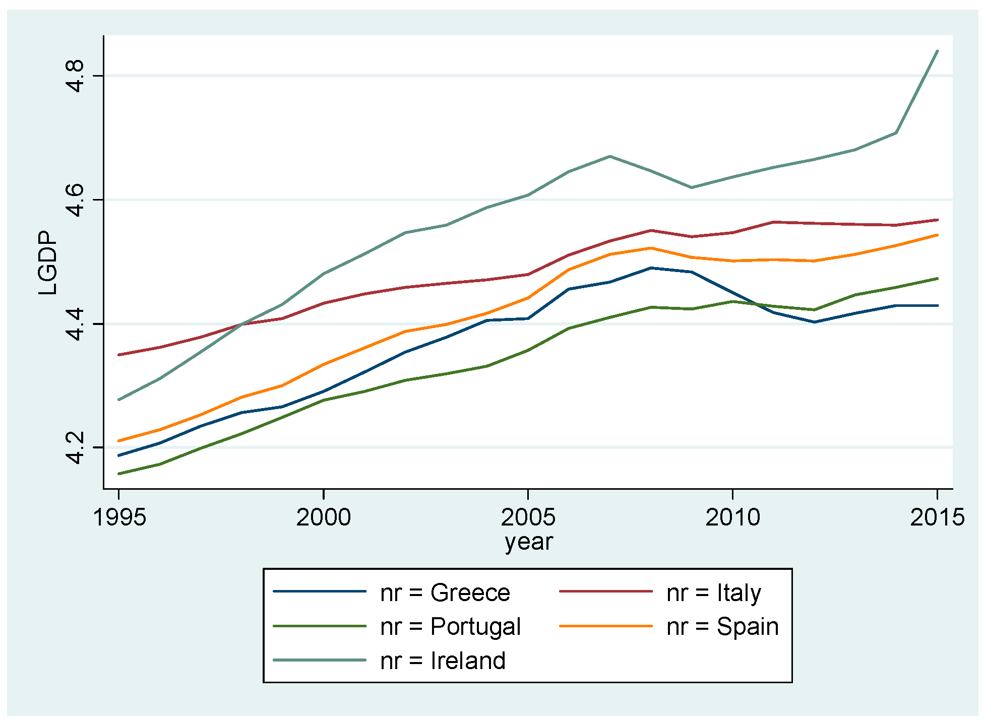
The effects of corruption, renewable energy, economic growth, and trade openness on carbon dioxide emissions are considered in this research. The methodology used in this study is panel data for the period 1995–2015, and we select the following European countries: Portugal, Spain, Italy, Ireland, and Greece. This group of countries have similar economic structures, namely in the distribution of per capita income, except for Ireland, which stands out from the other countries (Figure 1).
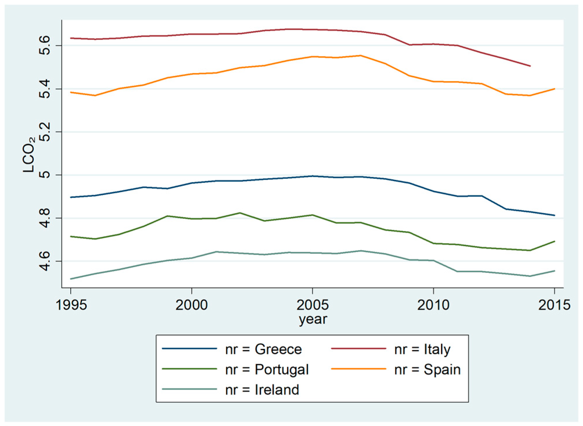
Thus, concerning the emission of carbon dioxide, it is observed that of the economies in question, Italy is the one that has the highest emissions of carbon dioxide, followed by Spain, Greece, and then Portugal and Ireland (Figure 2).
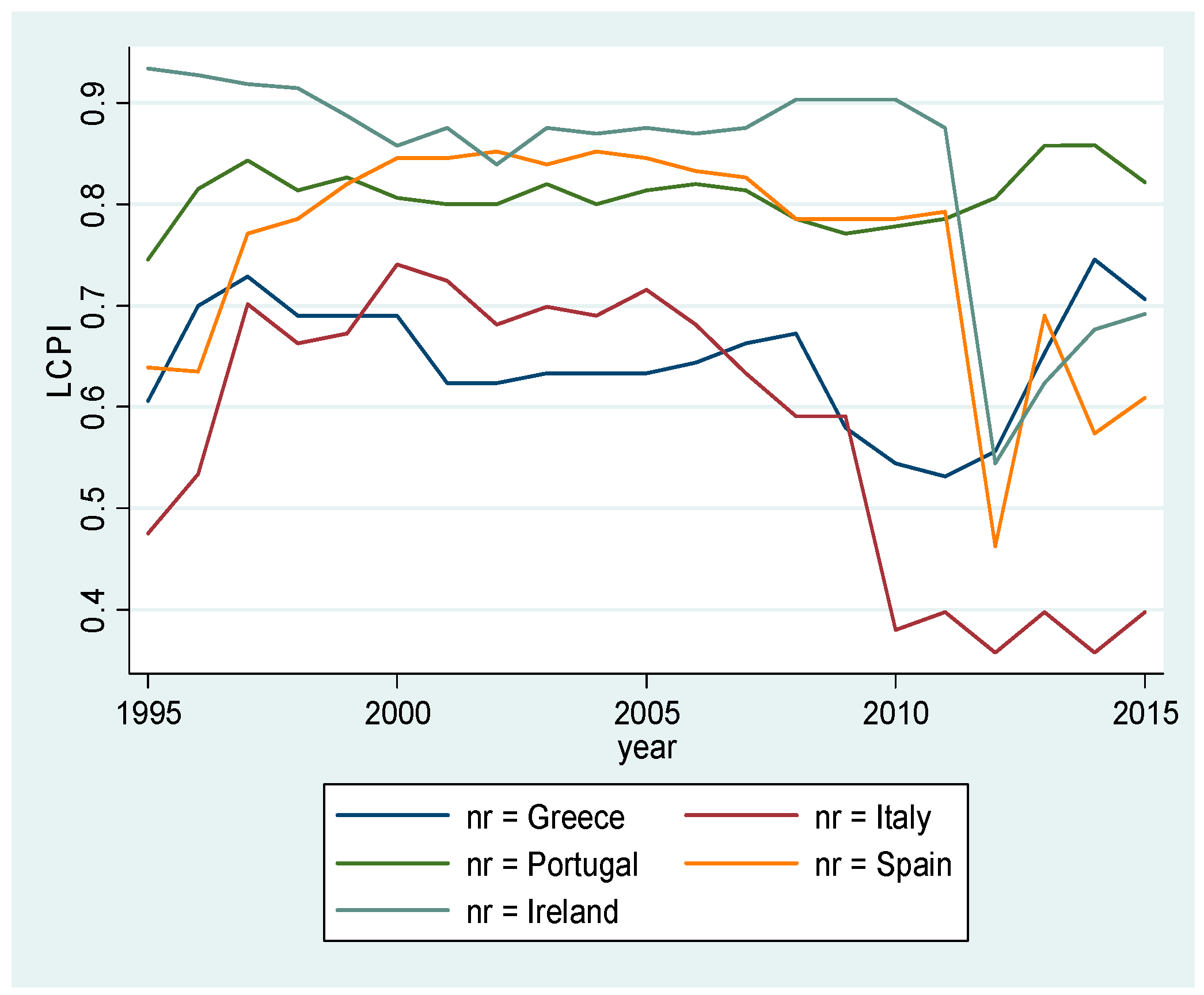
Regarding corruption, it is possible to infer that from 2010 onwards, there was an abrupt decline in all countries under analysis except for the Portuguese economy, which increased slightly (Figure 3).
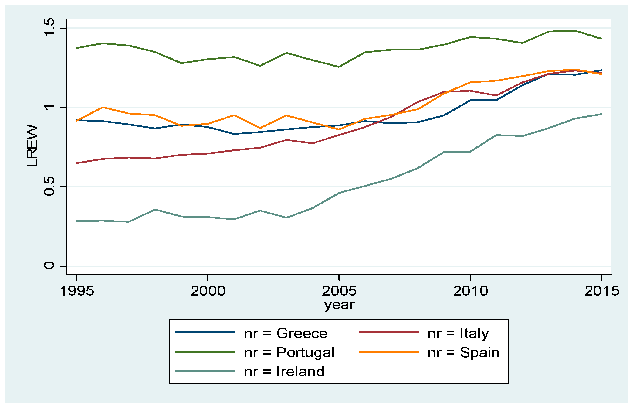
Concerning the use of renewable energies, it is observed that Portugal, of the economies under study, stands out in first place in terms of ranking. Ireland is one of the countries with less use of renewable energies; however, since 2005, there is an increasing trend towards the use of this type of energy (Figure 4).
The dependent variable evaluates the emissions of carbon dioxide (CO2) expressed in Kilotons. The independent variables are income per capita, corruption perception index, renewable energy, and exports of goods and services as a percentage of GDP. It should be mentioned that the data for the renewable energy variable is only available until 2015 from the World Bank (2021) data. On the other hand, the corruption perception index collected from the International Transparency database has only been available since 1995.
We started with unit root tests to assess whether the studies’ variables show stationarity or are integrated into the methodology’s first differences.
Then, we performed the multicollinearity test to see if we can specify the econometric model. Dumitrescu and Hurlin’s (2012) causality analysis were also considered to assess unidirectional and bidirectional causality among the variables used in this study. Regarding the econometric models used in this study, we applied the TSLS–Panel Two-Stage Least Squares (e.g., Anderson and Hsiao 1981, 1982; Arellano 1989; Arellano and Bond 1991) and panel cointegration (panel fully modified least-squares—FMOLS, panel dynamic least squares—DOLS, e.g., Saikkonen 1991; Phillips and Moon 1999).
Before applying the TSLS–Panel Two-Stage Least Squares estimator, it is necessary to apply the Hausman test to identify heterogeneity. The Hausman test compares random effects (RE) versus fixed effects (FE), indicating which estimators to use. After regression of the TSLS—Panel Two-Stage Least Squares model, it is necessary to apply the Breusch–Pagan postestimation test and the residual cross-section dependence test.
Therefore, the battery of panel unit root test such as Levin et al. (2002), ADF–Fisher Chi-square, Phillips–Perron, and Im et al. (2003) recommended by Maddala and Wu (1999), and Choi (2001) was applied to test and verify if the variables are stationary at the level or integrated into the first differences.
The next step pursued is to test the long-run panel data cointegration between the variables used in this study, considering Pedroni (2001, 2004) and the Kao (1999). As Leitão and Balsalobre-Lorente (2020) note, the Pedroni cointegration test is considered in two dimensions: with-dimension (panel cointegration) and between-dimension (mean panel). The panel v—statistics, panel rho—statistics, panel PP—statistics, and ADF—statistics represent the with-dimension. The classification between-dimension involves group rho—statistics, group PP—statistics, and group ADF—statistics.
Subsequently, the estimators of the panel fully modified least-squares (FMOLS) and panel dynamic least squares (DOLS) (e.g., Phillips and Hansen 1990; Stock and Watson 1993) are used to evaluate the long-run correlations between the variables used in this study.
Hypotheses and Model Specification
Considering the literature review, we formulate the following hypotheses:
Hypothesis 1 (H1).
Economic growth and economic activity are positively associated with carbon dioxide emissions.
This hypothesis is formulated from the assumptions of the Kuznets environmental curve and results from empirical studies of Bouyghrissi et al. (2021), Balsalobre-Lorente et al. (2019), Ike et al. (2020), Koengkan et al. (2021), and Leitão and Balsalobre-Lorente (2020). Most empirical studies find a positive impact between income per capita and carbon emissions, demonstrating that production and economic activity do not use clean energy and promote climate change and global warming.
The complexity of studying corruption and the different perspectives of this variable in the environment and climate change allows us to formulate two hypotheses as an alternative.
Hypothesis 2 (H2).
(a) Corruption causes adjustment costs in the environment; (b) the control of corruption reduces climate change.
This hypothesis was considered based on previous studies. As we analysed in the literature review, there are two different perspectives on the impact of corruption on carbon dioxide emissions: one of which argues that corruption’s control slows down climate change. However, as mentioned by the international transparency organization (https://www.transparency.org/en/what-is-corruption, accessed on 18 April 2021), corruption has impacts or costs in social, political, economic, and environmental terms. In this context, corruption accelerates carbon dioxide emissions, and environmental damage (e.g., Dincer and Fredriksson 2018; Ridzuan et al. 2019; Akhbari and Nejati 2019; Zhang and Chiu 2020).
According to the international transparency organization, the corruption index (CPI) is a perception index ranging from 0 to 10. The highest corruption corresponds to level 0, and the value 10 indicates the lowest level of corruption.
Hypothesis 3 (H3).
The use of renewable energy promotes sustainable development and air quality.
In recent years, empirical studies have argued that the replacement of nonrenewable energy with cleaner energy promotes the reduction of environmental costs, with a proliferation of studies that assess the causality between renewable energy and air quality. The studies by Maneejuk et al. (2020), Leitão and Balsalobre-Lorente (2020), Koengkan and Fuinhas (2020), and Balsalobre-Lorente et al. (2019) observed that there is a negative relationship with statistical significance between renewable energies and carbon dioxide emissions.
Hypothesis 4 (H4).
International trade aims to decrease climate change.
Regarding the arguments of the monopolistic competition models applied to international trade and the link with the environment, the empirical studies of Wang et al. (2018), Ike et al. (2020), Shahzad et al. (2021), and Leitão (2021) demonstrated that international trade is negatively correlated with carbon dioxide emissions. The authors state that trade is associated with sustainable practices which aim to reduce CO2 emissions. As Leitão and Balogh (2020) and Leitão (2021) argue, international trade allows us to explain innovation and product differentiation. In this context, innovation factors make it possible to reduce climate change and improve air quality.
Considering the studies of Zhang and Chiu (2020), Koengkan and Fuinhas (2020), Bouyghrissi et al. (2021), and Balsalobre-Lorente et al. (2019), the model assumes the following expression:
LCO2it = β0 + β1LGDPit + β2LCPIit + β3LREWit + β4LTOit + δt + ηi + εit
In this empirical study, we use as a dependent variable the logarithm of carbon dioxide emission (CO2) in kilotons to evaluate climate change, where i signifies the number of countries, and t signifies the time. Moreover, δt describes the common determinist trend, ηi are the specific effects, and εit represents the random disturbance.
The independent variables used in this study are the following:
- LGDP—represents the logarithm of income per capita expressed in USD.
- LCPI—signifies the logarithm of corruption perceptions index.
- LREW—indicates the logarithm of a percentage of renewable energy use in total final energy consumption.
- LTO—represents the logarithm of exports of goods and services in the percentage of GDP.
Table 1 presents the data, the expected signs considering the literature review and the sources used in this research.
4. Results and Discussion
This section exhibits the econometric results to test the relationship between corruption, economic growth, renewable energy, international trade, and carbon dioxide emissions (climate change).
Table 2 reveals the general statistics for all variables utilized in this empirical study. The variables of carbon dioxide emissions (LCO2) and income per capita (LGDP) represent the maximum’s higher values. Besides, the variables of carbon dioxide emissions (LCO2), income per capita (LGDP), and trade openness (LTO) present a positive skew. However, it is possible to observe that corruption index (LCPI) and renewable energy (LREW) exhibit a negative skew. The variable of carbon dioxide emissions (LCO2) presents the low kurtosis value, but the variable assumes the high value of standard deviation (std. dev).
Table 3 shows the unit root test results considering the methodology of Levin, Lin, and Chu, ADF–Fisher Chi-square, Phillips–Perron, and Im–Pesaran–Shin. Regarding the results, it is possible to infer that the variables of carbon dioxide emissions (LCO2), economic growth (LGDP), corruption index (LCPI), renewable energy (LREW), and trade openness (LTO) are stationary at the first difference I (1).
Table 4 illustrates the results of causality among the variables using the criterion of Dumitrescu–Hurlin pairwise causality.
We observe a unidirectional causality between economic growth (LGDP) and carbon dioxide emissions (LCO2). The linkages between carbon dioxide emissions (LCO2) and corruption (LCPI) and economic growth and corruption (LCPI) present a unidirectional causality. These results are according to the previous studies of Dincer and Fredriksson (2018), Ridzuan et al. (2019), and Lee et al. (2020). Besides, it is important to highlight that these results suggest that signs of the shadow economy occur and can be justified by the investigations of Bilan et al. (2020) and Nemec et al. (2021).
The same is valid between economic growth (LGDP) and renewable energy (LREW), and trade openness (LTO). The relationship between economic growth and renewable energies is based on sustainable economic development, which can be justified by the Kyoto Protocol (Kyoto Protocol to the United Nations Framework Convention on Climate Change 1997) and the Paris Agreement—UNFCCC (2015).
We also observe a unidirectional causality between renewable energy (LREW) and corruption (LCPI).
Furthermore, we see a bidirectional causality between renewable energy (LREW) and carbon dioxide emissions (LCO2). Our results also show a bidirectional causality between trade openness (LTO) and carbon dioxide emissions (LCO2).
Table 5 demonstrates the results of the panel cointegration test and Kao residual cointegration. According to the results, we can conclude that the variables are cointegrated in the long term. In this context, the results show a cointegration relationship between the variables economic growth, corruption, renewable energy, international trade, and carbon dioxide emissions.
Before proceeding with the model specification, it is necessary to perform the multicollinearity test and Hausman test to identify the endogeneity. First, it is essential to mention that multicollinearity is frequent through the OLS estimator or multiple linear regression model. As a rule, the independent variables have tolerance problems when VIF (variance inflation factor) is higher than five. According to the results in Table 6, we observe that all variables used in this research do not present a multicollinearity problem, VIF < 5.
When comparing random effects (RE) versus fixed effects (FE) using the Hausman test, Table 7 indicates that fixed effects are more appropriate.
Table 8 presents the econometric results with panel two-stage least squares (TSLS). We observe that economic growth (LGDP), renewable energy (LREW), and trade openness (LTO) are statistically significant at a 1% level. Moreover, the coefficient of corruption is statistically significant at a 10% level. In the Durbin–Watson statistics, we can refer that the estimates do not present problems of serial correlation. It is still possible to observe the Breusch–Pagan test in the present table, which admits homoscedasticity as a null hypothesis. The postestimation test presented confirms the presence of heteroscedasticity.
The variables of income per capita (LGDP) and corruption index (LCPI) are according to H1 and H2. The empirical result confirms that economic growth can generate environmental problems, which the Kuznets environmental curve’s assumptions can explain. Besides, the result obtained shows that corruption causes ecological and economic costs. The previous studies of Zhang and Chiu (2020), Arminen and Menegaki (2019), and Lee et al. (2020) give support to our results. Nevertheless, the coefficients of renewable energy (LREW) and trade openness (LTO) are negatively correlated with CO2 emissions, showing that clean energies and international trade promote sustainable development, and subsequently the improvements of environmental factors (e.g., Ahmed and Shimada 2019; Maneejuk et al. 2020; Razzaq et al. 2021; and Bouyghrissi et al. 2021).
Table 9 reports the estimates using the panel fully modified least squares (FMOLS) and panel dynamic ordinary least squares (DOLS).
According to our econometric results, it is possible to observe that the variables’ economic growth (LGDP) and trade openness (LTO) are statistically significant at the 1% level. These coefficients present a positive and negative impact on carbon dioxide emissions, respectively. Additionally, the renewable energy (LREW) variable is statistically significant at the 1% and 10% level with FMOLS (panel fully modified least squares) and DOLS (panel dynamic ordinary least squares).
The variable of corruption index (LCPI) presents a positive impact on CO2 emissions for both estimators with 10% and 5% levels, representing an increase in carbon dioxide emissions by 0.108% and 0.181%, respectively.
This result suggests that corruption can motivate climate change and environmental damage. The previous studies of Zhang and Chiu (2020), Lee et al. (2020), and Ridzuan et al. (2019) also found a positive impact of corruption on carbon dioxide emissions.
The coefficient of income per capita (LGDP) shows a positive impact on CO2 emissions. This result is according to the EKC hypothesis. The recent empirical studies of Balsalobre-Lorente et al. (2019), Ike et al. (2020), Koengkan et al. (2021), and Leitão and Balsalobre-Lorente (2020) also found a positive correlation between economic growth and carbon dioxide emissions.
The variable of renewable energy (LREW) is negatively correlated with carbon dioxide emissions showing that cleaner energies encourage environmental improvements. According to the results, the carbon dioxide emissions decreased (−0.189%) and (−0.126%). This result is in line with the various international conferences on the environment and climate issues and the EU Agenda (e.g., Kyoto Protocol to the United Nations Framework Convention on Climate Change 1997; Paris Agreement—UNFCCC 2015; Directive 2009/28/EC 2009). The empirical study is also supported by Koengkan and Fuinhas (2020) and Singh et al. (2019).
As the literature review reflects, trade openness (LTO) is negatively correlated with carbon dioxide emissions; our result found this association. The result can be explained by the trade intensity, as assessed by Leitão (2021), and this type of trade is associated with innovation and product differentiation. The empirical studies of Balsalobre-Lorente et al. (2021), Leitão and Balsalobre-Lorente (2020), Ike et al. (2020) also demonstrate that international trade present a negative effect on CO2 emissions. The authors concluded that international trade diminished climate change.
5. Conclusions
This study investigates the impacts of renewable energy, corruption perception, economic growth, and international trade on CO2 emissions considering panel data for 1995–2015. We selected five European economies: Portugal, Spain, Italy, Ireland, and Greece. We chose to focus on these countries because we intended to evaluate countries with relatively similar characteristics, as explained in this investigation’s introductiont. Besides, previous studies on this group of countries have not assessed the impact of corruption on climate issues.
The hypotheses were tested by panel unit root test (Levin et al. 2002; Choi 2001; Im et al. 2003). The results showed that the variables used in this research are stationary into the differences, I (1). Furthermore, the Pedroni and Kao panel cointegration demonstrated that the variables economic growth, corruption, renewable energy, international trade, and carbon dioxide emissions are cointegrated in the long run.
Regarding the Dumitrescu and Hurlin (2012) pairwise causality test, we conclude that, in general, the variables used in this empirical study present a unidirectional causality between them. The results still suggest a link between economic growth and corruption, showing signs of a shadow economy. However, we observe a bidirectional causality between renewable energy and carbon dioxide emissions. The same is verified by the relationship between international trade and carbon dioxide emissions.
The econometric results using TSLS (Panel Two-Stage Least Squares), FMOLS (panel Fully Modified Least Squares), and DOLS (panel Dynamic Least Squares) are similar between them.
The results found for the economic growth were in line with environmental Kuznets curve (EKC) studies. The empirical studies of Bouyghrissi et al. (2021), Balsalobre-Lorente et al. (2019), Ike et al. (2020), Koengkan et al. (2021), and Leitão and Balsalobre-Lorente (2020) also suggest that economic growth accelerates climate change and global warming.
The studies of Dincer and Fredriksson (2018), Ridzuan et al. (2019), Akhbari and Nejati (2019), Zhang and Chiu (2020) confirmed that corruption can accentuate pollution emissions, reflecting a policy of less transparency in terms of industrial and government policy. Our results in accordance with this perspective. Thus, a positive effect of corruption on CO2 emissions contains several economic and fiscal policy implications for government policies.
Subsequently, our econometric results also show that renewable energy and trade openness negatively correlated with carbon dioxide emissions. This result is according to the EU agenda, the Kyoto Protocol to the United Nations Framework Convention on Climate Change (1997), and the Paris Agreement—UNFCCC (2015), i.e., the concept of sustainable development (e.g., Balsalobre-Lorente et al. 2021; Leitão 2021).
Therefore, based on the empirical results, we can present some suggestions and implications for policymakers. First, the study shows that corruption can stimulate carbon dioxide emissions and, consequently, impacts environmental damage. Thus, governments and their finance ministries should implement more regulatory, supervisory, and corruption control measures, as this unfair practice distorts competition laws and policy. Second, the governments of the economies under analysis should continue to develop acceptable practices regarding decarbonization, promoting them as they have done with the introduction of renewable energies and more sustainable trade that considers innovation and differentiation.
Regarding the extent of this investigation and clues for future work, we think it would be interesting to compare these results with the BRICS (Brazil, Russia, India, China, and South Africa) economies since they are emerging economies with great potential for international trade. In this context, it will be essential to note that India has invested a lot in cleaner energy production in recent years. On the other hand, China has reversed its international trade patterns due to the current pandemic crisis and its response (e.g., Leitão and Balsalobre-Lorente 2020).
Funding
This research received no external funding.
Conflicts of Interest
The author declares no conflict of interest.
References
- Ahmed, Mun Mum, and Koji Shimada. 2019. The Effect of Renewable Energy Consumption on Sustainable Economic Development: Evidence from Emerging and Developing Economies. Energies 12: 2954. [Google Scholar] [CrossRef] [Green Version]
- Akhbari, Reza, and Mehdi Nejati. 2019. The effect of corruption on carbon emissions in developed and developing countries: Empirical investigation of a claim. Heliyon 5: e02516. [Google Scholar] [CrossRef] [Green Version]
- Alper, Aslan, and Ocal Oguz. 2016. The role of renewable energy consumption in economic growth: Evidence from asymmetric causality. Renewable and Sustainable Energy Reviews 60: 953–59. [Google Scholar] [CrossRef]
- Anderson, Theodore Wilbur, and Cheng Hsiao. 1981. Estimation of Dynamic Models with Error Components. Journal of the American Statistical Association 76: 598–606. [Google Scholar] [CrossRef]
- Anderson, Theodore Wilbur, and Cheng Hsiao. 1982. Formulation and Estimation of Dynamic Models using Panel Data. Journal of Econometrics 18: 47–82. [Google Scholar] [CrossRef]
- Arellano, Manuel. 1989. A note on the Anderson-Hsiao estimator for Panel Data. Economics Letters 31: 337–41. [Google Scholar] [CrossRef]
- Arellano, Manuel, and Stephen Bond. 1991. Some Tests of Specification for Panel Data: Monte Carlo Evidence and an Application to Employment Equations. The Review of Economic Studies 58: 277–97. [Google Scholar] [CrossRef] [Green Version]
- Arminen, Heli, and Angeliki N. Menegaki. 2019. Corruption, climate and the energy-environment-growth nexus. Energy Economics 80: 621–34. [Google Scholar] [CrossRef]
- Arnaut, Javier, and Johanna Lidman. 2021. Environmental Sustainability and Economic Growth in Greenland: Testing the Environmental Kuznets Curve. Sustainability 13: 1228. [Google Scholar] [CrossRef]
- Balsalobre-Lorente, Daniel, and Nuno Carlos Leitão. 2020. The role of tourism, trade, renewable energy use and carbon dioxide emissions on economic growth: Evidence of tourism-led growth hypothesis in EU-28. Environmental Science and Pollution Research 27: 45883–96. [Google Scholar] [CrossRef]
- Balsalobre-Lorente, Daniel, Muhammad Shahbaz, Charbel Jose Chiappetta Jabbour, and Oana M. Driha. 2019. The Role of Energy Innovation and Corruption in Carbon Emissions: Evidence Based on the EKC Hypothesis. In Energy and Environmental Strategies in the Era of Globalization Green Energy and Technology. Edited by Muhammad Shahbaz and Daniel Balsalobre. Cham: Springer, pp. 271–304. [Google Scholar]
- Balsalobre-Lorente, Daniel, Nuno Carlos Leitão, and Festus Victor Bekun. 2021. Fresh Validation of the Low Carbon Development Hypothesis under the EKC Scheme in Portugal, Italy, Greece and Spain. Energies 14: 250. [Google Scholar] [CrossRef]
- Bilan, Yuriy, Halyna Mishchuk, Natalia Samoliuk, and Halyna Yurchyk. 2020. Impact of Income Distribution on Social and Economic Well-Being of the State. Sustainability 12: 429. [Google Scholar] [CrossRef] [Green Version]
- Bouyghrissi, Soufiane, Berjaoui Abdelmoumen, and Maha Khanniba. 2021. The nexus between renewable energy consumption and economic growth in Morocco. Environmental Science and Pollution Research 28: 5693–5703. [Google Scholar] [CrossRef]
- Choi, In. 2001. Unit root tests for panel data. Journal of International Money and Finance 20: 249–72. [Google Scholar] [CrossRef]
- Cole, A. Matthew. 2007. Corruption, income and the environment: An empirical analysis. Ecological Economics 62: 637–47. [Google Scholar] [CrossRef]
- Dincer, Oguzhan C., and Per G. Fredriksson. 2018. Corruption and environmental regulatory policy in the United States: Does trust matter? Resource and Energy Economics 54: 212–25. [Google Scholar] [CrossRef]
- Directive 2009/28/EC of the European Parliament and of the Council of 23 April 2009 on the Promotion of the Use of Energy from Renewable Sources and Amending and Subsequently Repealing Directives 2001/77/EC and 2003/30/EC. 2009. Available online: https://eur-lex.europa.eu/legal-content/EN/ALL/?uri=CELEX%3A32009L0028 (accessed on 1 April 2021).
- Dumitrescu, Elena-Ivoana, and Christophe Hurlin. 2012. Testing for Granger non-causality in heterogeneous panels. Economic Modelling 29: 1450–60. [Google Scholar] [CrossRef] [Green Version]
- Grossman, Gene M., and Alan B. Krueger. 1991. Environmental impacts of a North American Free Trade Agreement. NBER Working Papers 3914. Cambridge: National Bureau of Economic Research, Inc. [Google Scholar]
- Grossman, Gene M., and Alan B. Krueger. 1995. Economic Growth and the Environment. The Quarterly Journal of Economics 110: 353–77. [Google Scholar] [CrossRef] [Green Version]
- Hassaballa, Hoda. 2015. The effect of corruption on carbon dioxide emissions in the Mena region. European Journal of Sustainable Development 4: 301–12. [Google Scholar] [CrossRef] [Green Version]
- Holtz-Eakin, Douglas, and Thomas M. Selden. 1995. Stoking the fires? CO2 Emissions and Economic Growth. Journal of Public Economics 1: 85–101. [Google Scholar] [CrossRef] [Green Version]
- Ibrahiem, Dalia M. 2015. Renewable Electricity Consumption, Foreign Direct Investment and Economic Growth in Egypt: An ARDL Approach. Procedia Economics and Finance 30: 313–23. [Google Scholar] [CrossRef] [Green Version]
- Ike, George N., Ojonugwa Usman, and Samuel Asumadu Sarkodie. 2020. Testing the role of oil production in the environmental Kuznets curve of oil producing countries: New insights from Method of Moments Quantile Regression. Science of Total Environment 711: 135208. [Google Scholar] [CrossRef] [PubMed]
- Im, Kyung So, M. Hashem Pesaran, and Yongcheol Shin. 2003. Testing for unit roots in heterogeneous panels. Journal of Econometrics 115: 53–74. [Google Scholar] [CrossRef]
- Kahia, Montassar, Anis Omri, and Bilel Jarraya. 2021. Green Energy, Economic Growth and Environmental Quality Nexus in Saudi Arabia. Sustainability 13: 1264. [Google Scholar] [CrossRef]
- Kao, Chihwa. 1990. Spurious regression and residual-based tests for cointegration in panel data. Journal of Econometrics 90: 1–44. [Google Scholar] [CrossRef]
- Karhan, Gökhan. 2019. Does Renewable Energy Increase Growth? Evidence from EU-19 Countries. International Journal of Energy Economics and Policy 9: 341–46. [Google Scholar]
- Khobai, Hlalefang, and Pierre Le Roux. 2018. Le Roux Does Renewable Energy Consumption Drive Economic Growth: Evidence from Granger-Causality Technique. International Journal of Energy Economics and Policy 8: 205–12. [Google Scholar]
- Koengkan, Matheus, and José Alberto Fuinhas. 2020. Exploring the Effect of the Renewable Energy Transition on CO2 Emissions of Latin American & Caribbean Countries. International Journal of Sustainable Energy 39: 515–38. [Google Scholar]
- Koengkan, Matheus, José Alberto Fuinhas, and Nuno Silva. 2021. Exploring the Capacity of Renewable Energy Consumption to Reduce Outdoor Air Pollution Death Rate in Latin America and the Caribbean Region. Environmental Science Pollution Research 28: 1656–74. [Google Scholar] [CrossRef]
- Kyoto Protocol to the United Nations Framework Convention on Climate Change. 1997. December 11. Available online: https://treaties.un.org/Pages/ViewDetails.aspx?src=IND&mtdsg_no=XXVII-7-a&chapter=27&clang=_en (accessed on 1 April 2021).
- Lee, Hui Shan, S. Y. Lee, Wai Mun Har, and C. W. Low. 2020. Energy Use and Corruption Mitigation: Implications for the Environmental Pollution. IOP Conf. Series: Earth and Environmental Science. Paper presented at the 5th International Conference on Civil and Environmental Engineering for Sustainability (IConCEES 2019), Le Grandeur Palm Resort, Johor, Malaysia, December 19–20. [Google Scholar]
- Leitão, Nuno Carlos. 2013. The environmental Kuznets curve and globalization: The Empirical Evidence for Portugal, Spain, Greece and Ireland. Energy Economics Letters 1: 15–23. [Google Scholar]
- Leitão, Nuno Carlos. 2021. Testing the role of trade on carbon dioxide emissions in Portugal. Economies 9: 22. [Google Scholar] [CrossRef]
- Leitão, Nuno Carlos, and Jeremiás Máté Balogh. 2020. The impact of intra-industry trade on carbon dioxide emissions: The case of the European Union. Agricultural Economics–Czech 66: 203–14. [Google Scholar] [CrossRef]
- Leitão, Nuno Carlos, and Daniel Balsalobre-Lorente. 2020. The Linkage between Economic Growth, Renewable Energy, Tourism, CO2 Emissions, and International Trade: The Evidence for the European Union. Energies 13: 4838. [Google Scholar] [CrossRef]
- Levin, Andrew, Chien-Fu Lin, Chia-Shang, and James Chu. 2002. Unit Root Test in Panel Data: Asymptotic and Finite Sample Properties. Journal of Econometrics 108: 1–24. [Google Scholar] [CrossRef]
- Maddala, Gangadharrao S., and Shaowen Wu. 1999. A comparative study of unit root tests with panel data and a new simple test. Oxford Bulletin of Economics and Statistics 61: 631–52. [Google Scholar] [CrossRef]
- Mahmoodi, Majid. 2017. The Relationship between Economic Growth, Renewable Energy, and CO2 Emissions: Evidence from Panel Data Approach. International Journal of Energy Economics and Policy 7: 96–102. [Google Scholar]
- Maneejuk, Nutnaree, Sutthipat Ratchakom, Paravee Maneejuk, and Woraphon Yamaka. 2020. Does the Environmental Kuznets Curve Exist? An International Study. Sustainability 12: 9117. [Google Scholar] [CrossRef]
- Marinaş, Marius-Corneliu, Marin Dinu, Aura-Gabriela Socol, and Cristian Socol. 2018. Renewable Energy Consumption and Economic Growth. Causality Relationship in Central and Eastern European countries. PLoS ONE 13: e0202951. [Google Scholar] [CrossRef] [Green Version]
- Masron, Tajul Ariffin, and Yogeeswari Subramaniam. 2018. The environmental Kuznets curve in the presence of corruption in developing countries. Environmental Science and Pollution Research 25: 12491–506. [Google Scholar] [CrossRef]
- Nemec, Daniel, Eva Kotlánová, Igor Kotlán, and Zuzana Machová. 2021. Corruption, Taxation and the Impact on the Shadow Economy. Economies 9: 18. [Google Scholar] [CrossRef]
- Paris Agreement—UNFCCC. 2015. Available online: https://unfccc.int/sites/default/files/english_paris_agreement.pdf (accessed on 18 April 2021).
- Pedroni, Peter. 2001. Purchasing power parity tests in cointegrated panels. The Review of Economics and Statistic 83: 727–31. [Google Scholar] [CrossRef] [Green Version]
- Pedroni, Peter. 2004. Panel cointegration: Asymptotic and finite sample properties of pooled time series tests with an application to the PPP hypothesis. Econometric Theory 20: 597–625. [Google Scholar] [CrossRef] [Green Version]
- Phillips, Peter C. B., and Bruce E. Hansen. 1990. Statistical Inference in Instrumental Variables Regression with I (1) Processes. Review of Economic Studies 57: 99–125. [Google Scholar] [CrossRef]
- Phillips, Peter C. B., and Hyungsik R. Moon. 1999. Linear Regression Limit Theory for Nonstationary Panel Data. Econometrica 67: 1057–111. [Google Scholar] [CrossRef] [Green Version]
- Rahman, Habib Ur, Umer Zaman, and Jarosław Górecki. 2021. The Role of Energy Consumption, Economic Growth and Globalization in Environmental Degradation: Empirical Evidence from the BRICS Region. Sustainability 13: 1924. [Google Scholar] [CrossRef]
- Razzaq, Naveed, Faqeer Muhammad, Rehmat Karim, Muhammad Tariq, and Khair Muhammad. 2021. The Nexus between Energy, Environment and Growth: Evidence from Latin-American Countries. International Journal of Economics and Policy 11: 82–87. [Google Scholar]
- Ridzuan, Abdul Rahim, Noraina Mazuin Sapuan, Nur Hayati Abd Rahman, Halimahton Borhan, and Azhana Othman. 2019. The Impact of Corruption on Environmental Quality in the Developing Countries of ASEAN-3: The Application of the Bound Test. International Journal of Energy Economics and Policy 9: 469–78. [Google Scholar] [CrossRef]
- Sahlia, Ikram, and Jaleleddine Ben Rejeb. 2015. The environmental Kuznets curve and corruption in the Mena region. Procedia-Social and Behavioral Sciences 195: 1648–57. [Google Scholar] [CrossRef] [Green Version]
- Saikkonen, Pentti. 1991. Asymptotically Efficient Estimation of Cointegration Regressions. Econometric Theory 7: 1–21. [Google Scholar] [CrossRef]
- Sansyzbayeva, Galiya, Zhansaya Temerbulatova, Zhidebekkyzy Aknur, and Ashirbekova Laura. 2020. Evaluating the transition to green economy in Kazakhstan: A synthetic control approach. Journal of International Studies 13: 324–41. [Google Scholar] [CrossRef] [PubMed]
- Saputra, Putu Mahardika Adi. 2019. Corruption perception and bilateral trade flows: Evidence from developed and developing countries. Journal of International Studies 12: 65–78. [Google Scholar] [CrossRef] [Green Version]
- Sekrafi, Habib, and Asma Sghaier. 2018. The effect of corruption on carbon dioxide emissions and energy consumption in Tunisia. PSU Research Review: An International Journal 2: 81–95. [Google Scholar] [CrossRef] [Green Version]
- Shahbaz, Muhammad, Farooq Ahmed Jam, Sadia Bibi, and Nanthakumar Loganathan. 2016. Multivariate Granger Causality between CO2 Emissions, Energy intensity and Economic Growth in Portugal: Evidence from Cointegration and Causality Analysis. Technological and Economic Development of Economy 22: 47–74. [Google Scholar] [CrossRef]
- Shahzad, Umer, Buhari Doğan, Avik Sinha, and Zeeshan Fareed. 2021. Does Export product diversification help to reduce energy demand: Exploring the contextual evidences from the newly industrialized countries. Energy 214: 118881. [Google Scholar] [CrossRef]
- Singh, Nadia, Richard Nyuur, and Ben Richmond. 2019. Renewable Energy Development as a Driver of Economic Growth: Evidence from Multivariate Panel Data Analysis. Sustainability 11: 2418. [Google Scholar] [CrossRef] [Green Version]
- Soava, Georgeta, Anca Mehedintu, Mihaela Sterpu, and Mircea Radutean. 2018. Impact of Renewable Energy Consumption on Economic Growth: Evidence from European Union Countries. Technological and Economic Development of Economy 24: 914–32. [Google Scholar] [CrossRef]
- Sriyana, Jaka. 2019. Effects of Energy Consumption on Economic Growth in an Emerging Economy. International Journal of Energy Economics and Policy 9: 283–90. [Google Scholar] [CrossRef]
- Stock, James, and Mark Watson. 1993. Simple Estimation of Cointegration Vectors in Higher Order Integrated Systems. Econometrica 61: 783–820. [Google Scholar] [CrossRef]
- Wang, Zhaohua, Danish, Bin Zhang, and Bo Wang. 2018. The moderating role of corruption between economic growth and CO2 emissions: Evidence from BRICS economies. Energy 148: 506–13. [Google Scholar] [CrossRef]
- Zhang, Wenwen, and Yi-Bin Chiu. 2020. Do country risks influence carbon dioxide emissions? A non-linear perspective. Energy 206: 118048. [Google Scholar] [CrossRef]
Figure 1.
Panel data line plot of income per capita.

Figure 2.
Panel data line plot of carbon dioxide emissions.

Figure 3.
Panel data line plot of corruption index.

Figure 4.
Panel data line renewable energy.


Table 1.
Data, Expected Signs, and Sources.
| Data | Expected Signs | Source |
|---|---|---|
| LCO2—Logarithm of carbon dioxide emissions in kilotons | World Bank–World Development Indicators (2021), and Carbon Dioxide Information Analysis Center. | |
| LGDP—Logarithm of income per capita based on purchasing power parity (PPP) | [+] | World Bank–World Development Indicators (2021), and OECD National Account. |
| LCPI—Logarithm of corruption perceptions index | [+] | Transparency International, CPI—Corruption Perception Index data. |
| LREW—Logarithm of a percentage of renewable energy use | [−] | World Bank–World Development Indicators (2021), and International Energy Agency. |
| LTO—Logarithm of exports of goods in percentage of GDP | [−] | World Bank–World Development Indicators (2021), and OECD National Account. |
Table 2.
Descriptive Statistics.
| LCO2 | LGDP | LCPI | LREW | LTO | |
|---|---|---|---|---|---|
| Mean | 5.065 | 4.433 | 0.728 | 0.953 | 1.5211 |
| Median | 4.940 | 4.430 | 0.758 | 0.929 | 1.433 |
| Maximum | 5.676 | 4.839 | 0.933 | 1.484 | 2.086 |
| Minimum | 4.518 | 4.157 | 0.358 | 0.279 | 1.155 |
| Std. Dev. | 0.407 | 0.132 | 0.136 | 0.316 | 0.233 |
| Skewness | 0.272 | 0.158 | −0.806 | −0.398 | 1.126 |
| Kurtosis | 1.440 | 2.983 | 3.1923 | 2.5962 | 3.009 |
| Probability | 0.003 | 0.806 | 0.003 | 0.178 | 0.000 |
| Observations | 104 | 104 | 104 | 104 | 104 |
Notes: All variables are in logarithmic form.
Table 3.
Panel Unit Root Test.
| Variables | Level | First Difference | ||
|---|---|---|---|---|
| Carbon Dioxide Emissions | LCO2 | DLCO2 | ||
| Method | Statistic | p-value | Statistic | p-value |
| Levin, Lin and Chu t | −0.821 | (0.206) | −3.890 *** | (0.000) |
| ADF—Fisher Chi-square | 6.821 | (0.742) | 25.925 *** | (0.003) |
| PP—Fisher Chi-square | 7.583 | (0.669) | 48.315 *** | (0.000) |
| IPS-Im, Pesaran, Shin W-Stat | 2.088 | (0.982) | −1.393 * | (0.081) |
| Level | First difference | |||
| Income per capita | LGDP | DLGDP | ||
| Method | Statistic | p-value | Statistic | p-value |
| Levin, Lin and Chu t | 3.562 | (0.999) | −2.772 *** | (0.003) |
| ADF—Fisher Chi-square | 0.474 | (1.000) | 17.121 * | (0.071) |
| PP—Fisher Chi-square | 0.048 | (1.000) | 19.552 ** | (0.034) |
| IPS-Im, Pesaran, Shin W-Stat | 1.374 | (0.915) | 0.029 | (0.512) |
| Level | First difference | |||
| Corruption Index | LCPI | DLCPI | ||
| Method | Statistic | p-value | Statistic | p-value |
| Levin, Lin and Chu t | −0.659 | (0.254) | −8.233 *** | (0.000) |
| ADF—Fisher Chi-square | 7.142 | (0.712) | 69.599 *** | (0.000) |
| PP—Fisher Chi-square | 6.499 | (0.771) | 95.413 *** | (0.000) |
| IPS-Im, Pesaran, Shin W-Stat | −0.934 | (0.175) | −4.935 *** | (0.000) |
| Level | First difference | |||
| Renewable Energy | LREW | DLREW | ||
| Method | Statistic | p-value | Statistic | p-value |
| Levin, Lin and Chu t | 2.615 | (0.995) | −4.735 *** | (0.000) |
| ADF—Fisher Chi-square | 0.903 | (0.999) | 40.613 *** | (0.000) |
| PP—Fisher Chi-square | 0.566 | (1.000) | 69.882 *** | (0.000) |
| IPS-Im, Pesaran, Shin W-Stat | 3.997 | (1.000) | −3.353 *** | (0.000) |
| Level | First difference | |||
| Trade Openness | LTO | DLTO | ||
| Method | Statistic | p-value | Statistic | p-value |
| Levin, Lin and Chu t | 2.310 | (0.989) | −6.339 *** | (0.000) |
| ADF—Fisher Chi-square | 0.847 | (0.999) | 52.042 *** | (0.000) |
| PP—Fisher Chi-square | 0.340 | (1.000) | 62.034 *** | (0.000) |
| IPS-Im, Pesaran, Shin W-Stat | 1.075 | (0.858) | −3.901 *** | (0.000) |
Notes: ***, **, and * represent statistically significant at 1%, 5%, 10% levels. All variables are in logarithmic form.
Table 4.
Dumitrescu–Hurlin pairwise causality test.
| Null Hypothesis: | W-Stat. | Zbar-Stat. | Prob. |
|---|---|---|---|
| LGDP does not homogeneously cause LCO2 | 11.043 *** | 7.008 | (0.000) |
| LCO2 does not homogeneously cause LGDP | 2.599 | 0.2098 | (0.833) |
| LCPI does not homogeneously cause LCO2 | 3.811 | 1.1850 | (0.237) |
| LCO2 does not homogeneously cause LCPI | 5.623 *** | 2.6437 | (0.008) |
| LREW does not homogeneously cause LCO2 | 9.192 *** | 5.5174 | (0.000) |
| LCO2 does not homogeneously cause LREW | 6.458 *** | 3.3167 | (0.000) |
| LTO does not homogeneously cause LCO2 | 6.438 *** | 3.000 | (0.001) |
| LCO2 does not homogeneously cause LTO | 6.088 *** | 3.019 | (0.002) |
| LCPI does not homogeneously cause LGDP | 2.158 | −0.142 | (0.887) |
| LGDP does not homogeneously cause LCPI | 6.147 *** | 3.089 | (0.002) |
| LREW does not homogeneously cause LGDP | 1.227 | −0.896 | (0.370) |
| LGDP does not homogeneously cause LREW | 9.199 *** | 5.561 | (0.000) |
| LTO does not homogeneously cause LGDP | 2.075 | −0.209 | (0.834) |
| LGDP does not homogeneously cause LTO | 5.115 ** | 2.253 | (0.024) |
| LREW does not homogeneously cause LCPI | 11.572 *** | 7.4823 | (0.000) |
| LCPI does not homogeneously cause LREW | 4.192 | 1.505 | (0.132) |
| LTO does not homogeneously cause LCPI | 3.970 | 1.326 | (0.185) |
| LCPI does not homogeneously cause LTO | 4.321 | 1.6099 | (0.107) |
| LREW does not homogeneously cause LTO | 2.910 | 0.467 | (0.640) |
| LTO does not homogeneously cause LREW | 8.045 *** | 4.626 | (0.000) |
Notes: ***, and ** represent statistically significant at 1%, 5%, levels. All variables are in logarithmic form.
Table 5.
Panel Cointegration Test Results with Intercept and Trend.
| (Within Dimension) | ||||
|---|---|---|---|---|
| Weighted | ||||
| Statistic | Prob. | Statistic | Prob. | |
| Panel v-Statistic | 1.4048 ** | (0.080) | 1.4159 * | (0.078) |
| Panel rho-Statistic | 0.277 | (0.609) | 0.279 | (0.610) |
| Panel PP-Statistic | −1.801 ** | (0.036) | −1.762 ** | (0.039) |
| Panel ADF-Statistic | −2.529 *** | (0.005) | −2.498 *** | (0.006) |
| (Between-Dimension) | ||||
| Statistic | Prob. | |||
| Group rho-Statistic | 1.150 | (0.875) | ||
| Group PP-Statistic | −2.211 ** | (0.014) | ||
| Group ADF-Statistic | −2.489 *** | (0.006) | ||
| t-Statistic | Prob. | |||
| ADF | −2.243 ** | (0.013) | ||
| Residual variance | 0.000637 | |||
| Heteroskedasticity- and autocorrelation-consistent (HAC) variance | 0.000582 | |||
Notes: ***, **, and * represent statistically significant at 1%, 5%, 10 levels.
Table 6.
Testing the Multicollinearity Based on OLS Estimator.
| Variables | VIF | 1/VIF |
|---|---|---|
| LGDP | 2.07 | 0.4836 |
| LCPI | 1.62 | 0.616 |
| LREW | 1.29 | 0.778 |
| LTO | 2.83 | 0.3534 |
| Mean VIF | 1.95 |
Notes: All variables are in logarithmic form.
Table 7.
Hausman test.
| Chi-Sq. Statistic (4) = 30.990 *** |
Notes: H0 = random effects (RE) versus fixed effects (FE), *** represents statistically significant at 1% level.
Table 8.
Panel Two-Stage Least Squares.
| Variables | TSLS Coef. |
|---|---|
| LGDP | 0.393 *** (0.000) |
| LCPI | 0.062 * (0.056) |
| LREW | −0.246 *** (0.000) |
| LTO | −0.338 *** (0.000) |
| Constant | 4.025 *** (0.000) |
| SE of regression | 0.032 |
| Mean dep var | 5.065 |
| S.D dep var | 0.407 |
| Durbin–Watson stat | 0.412 |
| Sum squ. resi. | 0.095 |
| Breusch–Pagan | 32.814 *** |
| Sum squ. resi. | 0.095 |
| Observations | 104 |
Notes: ***, and * represent statistically significant at 1%, 10% levels. All variables are in logarithmic form.
Table 9.
Panel Fully Modified Least Squares and Panel Dynamic Least Squares.
| Variables | FMOLS Coef. | DOLS Coef. |
|---|---|---|
| LGDP | 0.365 *** (0.000) | 0.387 *** (0.000) |
| LCPI | 0.108 * (0.085) | 0.181 ** (0.027) |
| LREW | −0.189 *** (0.000) | −0.126 * (0.059) |
| LTO | −0.448 *** (0.000) | −0.505 *** (0.000) |
| SE of regression | 0.032 | 0.017 |
| Long-run var | 0.002 | 0.000 |
| Mean dep var | 5.067 | 5.078 |
| S.D dep var | 0.406 | 0.469 |
| Sum squ. resi. | 0.092 | 0.006 |
| Observations | 99 | 99 |
Notes: ***, **, and * represent statistically significant at 1%, 5%, 10% levels. All variables are in logarithmic form.
Publisher’s Note: MDPI stays neutral with regard to jurisdictional claims in published maps and institutional affiliations. |
© 2021 by the author. Licensee MDPI, Basel, Switzerland. This article is an open access article distributed under the terms and conditions of the Creative Commons Attribution (CC BY) license (https://creativecommons.org/licenses/by/4.0/).
Share and Cite
MDPI and ACS Style
Leitão, N.C. The Effects of Corruption, Renewable Energy, Trade and CO2 Emissions. Economies 2021, 9, 62. https://doi.org/10.3390/economies9020062
AMA Style
Leitão NC. The Effects of Corruption, Renewable Energy, Trade and CO2 Emissions. Economies. 2021; 9(2):62. https://doi.org/10.3390/economies9020062
Chicago/Turabian StyleLeitão, Nuno Carlos. 2021. "The Effects of Corruption, Renewable Energy, Trade and CO2 Emissions" Economies 9, no. 2: 62. https://doi.org/10.3390/economies9020062
Note that from the first issue of 2016, this journal uses article numbers instead of page numbers. See further details here.