Effect of Battery Electric Vehicles on Greenhouse Gas Emissions in 29 European Union Countries

Abstract

This analysis explored the effect of battery electric vehicles (BEVs) on greenhouse gas emissions (GHGs) in a panel of twenty-nine countries from the European Union (EU) from 2010 to 2020. The method of moments quantile regression (MM-QR) was used, and the ordinary least squares with fixed effects (OLSfe) was used to verify the robustness of the results. The MM-QR support that in all three quantiles, economic growth causes a positive impact on GHGs. In the 50th and 75th quantiles, energy consumption causes a positive effect on GHGs. BEVs in the 25th, 50th, and 75th quantiles have a negative impact on GHGs. The OLSfe reveals that economic growth has a negative effect on GHGs, which contradicts the results from MM-QR. Energy consumption positively impacts GHGs. BEVs negatively impacts GHGs. Although the EU has supported a more sustainable transport system, accelerating the adoption of BEVs still requires effective political planning to achieve net-zero emissions. Thus, BEVs are an important technology to reduce GHGs to achieve the EU targets of decarbonising the energy sector. This research topic can open policy discussion between industry, government, and researchers, towards ensuring that BEVs provide a climate change mitigation pathway in the EU region.

1. Introduction

The arguments for climate protection have never been so convincing as now. Globally, climate change is endangering the lives of millions of people and threatening many aspects of the human economy [1]. The transport sector is expected to be a crucial part of the solution: a sector that can help reduce greenhouse gas (GHG) emissions, including carbon dioxide (CO₂) and non-CO₂ gases such as methane (CH₄), nitrous oxide (N₂O), partially fluorinated hydrocarbons (HFC), perfluorinated hydrocarbons (PFC), sulfur hexafluoride (SF6), and nitrogen trifluoride (NF3). To a greater or lesser extent, these gases are harmful to the environment as they trap heat in the atmosphere, causing global warming [2].

Climate change and the contemporary transportation system are inextricably linked in many ways. The Industrial Revolution innovations that brought in new forms of transportation are the same technologies that have led to the increasing GHGs in the atmosphere [3]. The need for fossil fuels such as coal and oil surged as machines replaced manual labour in the second half of the 18th century [3]. Powerful modern mobility, such as vehicles, steam-powered trains, and boats, were all powered by fossil fuels, which emit significant volumes of CO₂ into the atmosphere when combusted [4]. 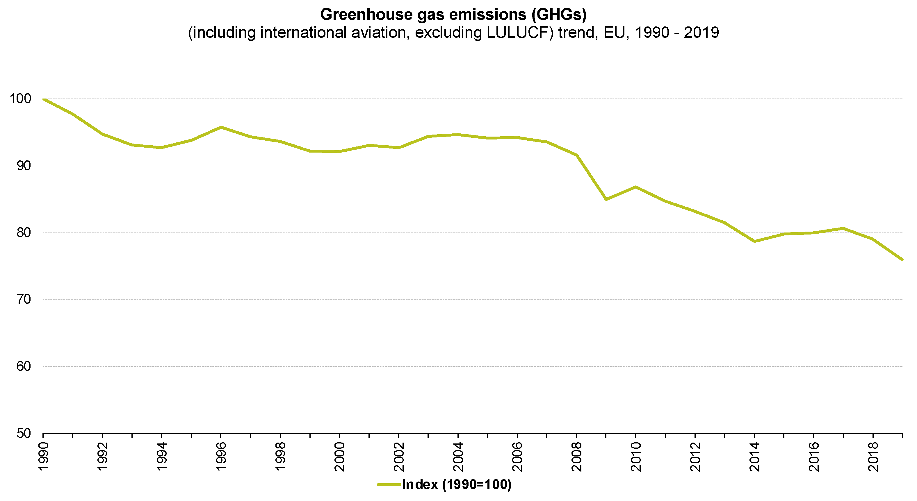As recent evidence showed, CO₂ levels rose and resulted in a significant greenhouse effect [5]. Given the transport sector’s potential, the hotly discussed transport-related environmental problem is how to fulfil the growing need for increased global connection and mobility sustainably. This study looks at the latest developments in the European Union (EU). In general, (GHG) emissions in the EU have been gradually declining in recent years, wherein 2019, the GHG emissions in the EU were down by (24%) compared with 1990 levels, representing an absolute reduction of 1182 million tonnes of CO₂-equivalents (see Figure 1 below).

As shown in Figure 1 above, from 1999 to 2008, the progression of GHGs emissions in the EU was unchanged. Moreover, in 2009, the GHGs emissions dropped due to the global financial and economic crisis and reduced industrial activity. However, the emissions increased in 2010 and decreased again from 2011 onward. Between 2015 to 2017, these emissions had slightly been increasing. In 2019, emissions decreased by (3.8%) (149 million tonnes of CO₂-equivalents) compared to 2018 levels [6].

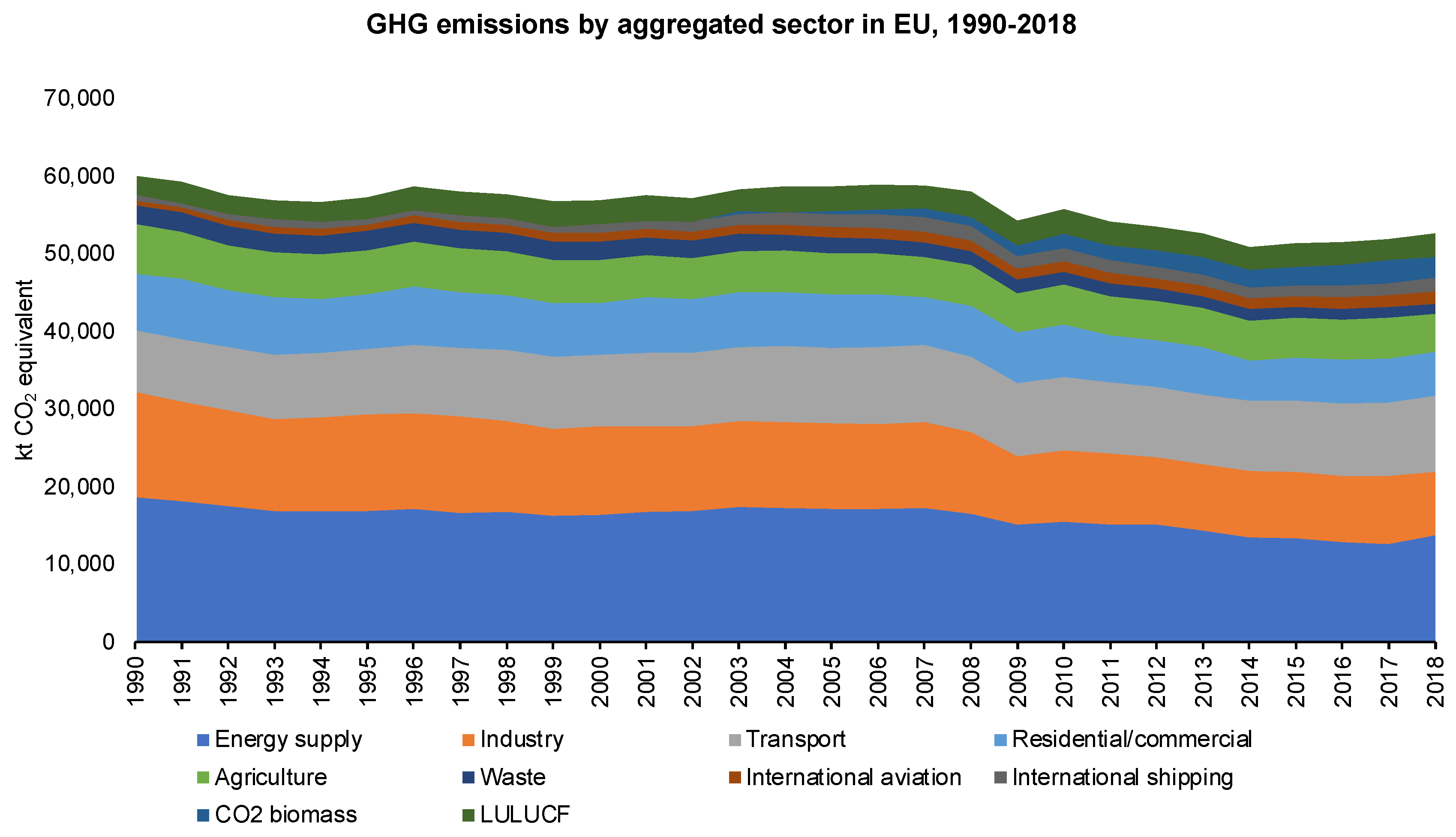
In the EU, the energy-producing industries sector was the most significant contributor to the increase of GHG emissions, where the sector contributed with (28.0%), followed by fuel combustion by users (25.5%) and the transport sector (24.6%). Indeed, compared with 1990, the share of most sources decreased, transport increased from (14.8%) in 1990 to (24.6%) in 2018 (see Figure 2 below).

Indeed, the GHG emissions from the majority of sector decrease between 1990 to 2018 (e.g., Energy supply (−32%); Industry (−35%); Residential/commercial (−22%); Agriculture (−19%); and Waste (−42%)) with exception of the transport sector that registered an increase of (+19%). Moreover, the largest decrease in emissions in absolute terms occurred in energy supply and industry. However, agriculture, residential and commercial, and waste management have decreased GHG emissions since 1990 (see Figure 3 below).

Moreover, Figure 3 above also shows an increase in GHGs from biomass combustion (+182%), international aviation (+129%), and international shipping (+32%). Although net removals from land use, land-use change and forestry (LULUCF) increased over the period, the substantial increase in GHGs from biomass combustion highlights the rapidly growing use of biomass in replacing fossil fuel sources in the EU [6].

Although intervention is needed in all sectors to meet emission reduction targets, it is crucial to reduce the emissions, particularly from the transport sector in the EU, where the GHGs from this sector increased by (19%). Therefore, reducing transport related GHG emissions is projected to be especially difficult, but emerging technologies have the potential to make significant contributions to GHG mitigation in the sector (e.g., Hawkins et al. [8]; and Andersson and Börjesson [9]). Reducing vehicle energy and fuel carbon intensities offers the best potential for European countries to achieve significant reductions in GHG emissions from vehicular transportation (e.g., Xu et al. [10]; and Andersson and Börjesson, [9]).

The thermodynamics of traditional internal combustion engine vehicles (ICEVs) severely limit their energy efficiency potential, increasing the necessity for fossil fuel use in transportation (e.g., Hawkins et al. [8]: Helmers and Marx [11]; and Tagliaferri et al. [12]). Battery electric vehicles (BEVs) have recently been viewed as a viable alternative to ICEVs but have only recently inspired considerable public interest and acceptance (e.g., Ajanovic and Haas [13]). BEVs have a more efficient powertrain, require less maintenance, and generate no exhaust pollutants (e.g., Hawkins et al. [8] and Bekel and Pauliuk [14]). Because of these features, BEVs are viewed as a strong contender for reducing transportation related GHG and air pollutant emissions (Hawkins et al. [8]). However, mitigation efficacy may be limited by emissions from battery production and charging requirements (Andersson and Börjesson [9]).

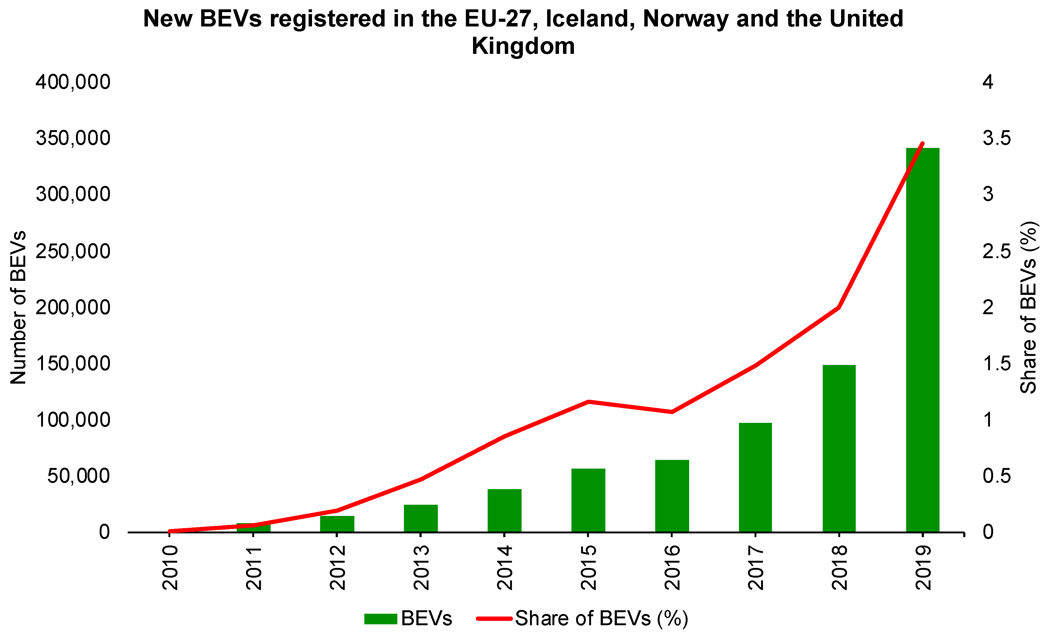
In the EU, the BEVs are gradually penetrating the market. However, despite a steady increase in the number of new electric car registrations annually, from 734 units in 2010 to about 341,267 units in 2019, they still account for a market share of only (3.46%) of newly registered passenger vehicles (see Figure 4 below).

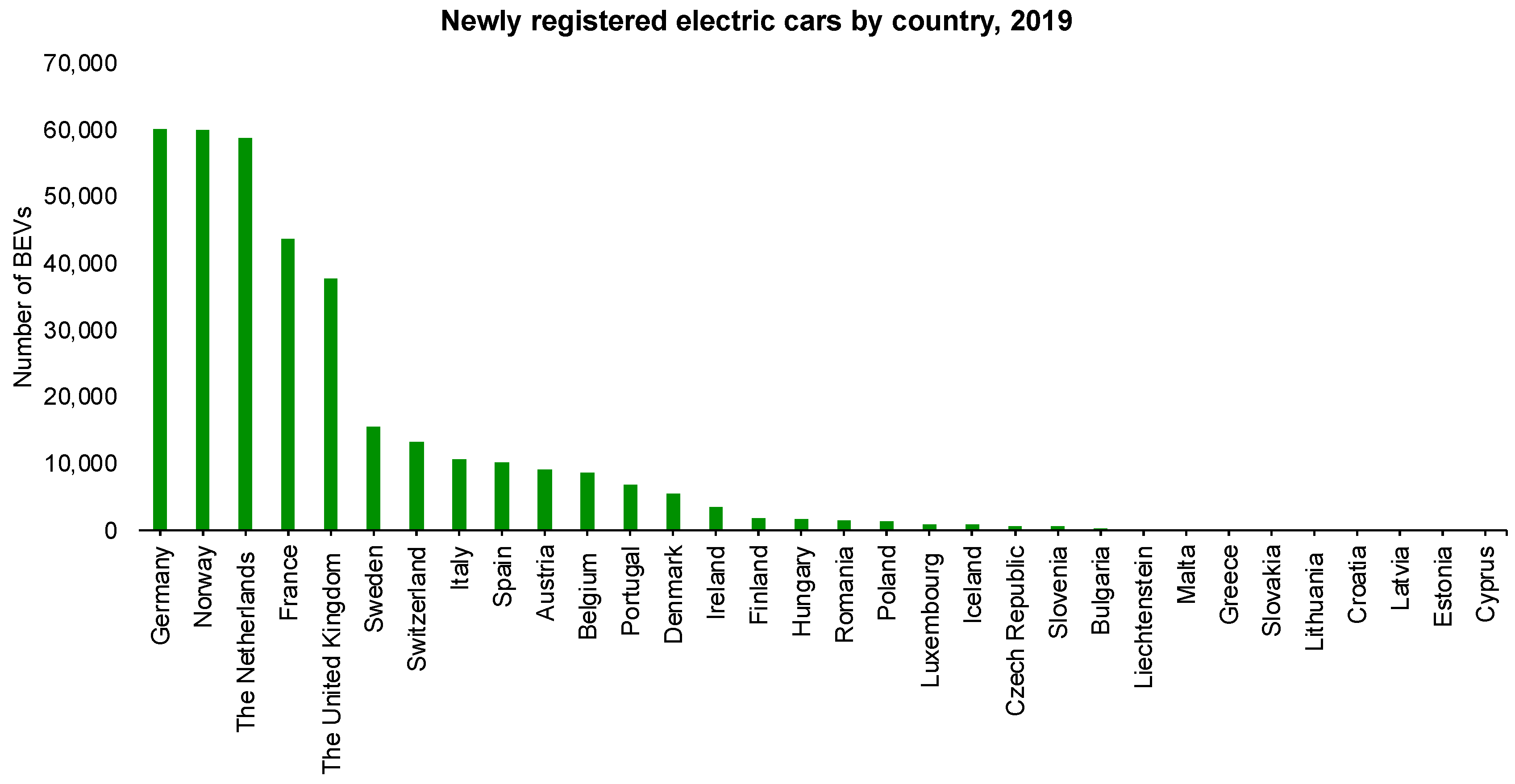
Figure 4 above shows that the number of new BEVs registered in the EU is increasing. Indeed, more than half of all BEVs registrations were in Germany, Norway, the Netherlands, France, and the United Kingdom (see Figure 5 below).

In some countries, such as Cyprus, Estonia, Greece, Lithuania, Slovakia, and Slovenia, the proportion of BEVs in total vehicle registration remained below 200 units in 2019. On the other hand, there was a notable increase in new BEV registrations between 2018 and 2019 (129%), which can be partly explained by the inclusion of Norway in the data set in 2019, a country that registered around 60,000 BEVs that year [6].

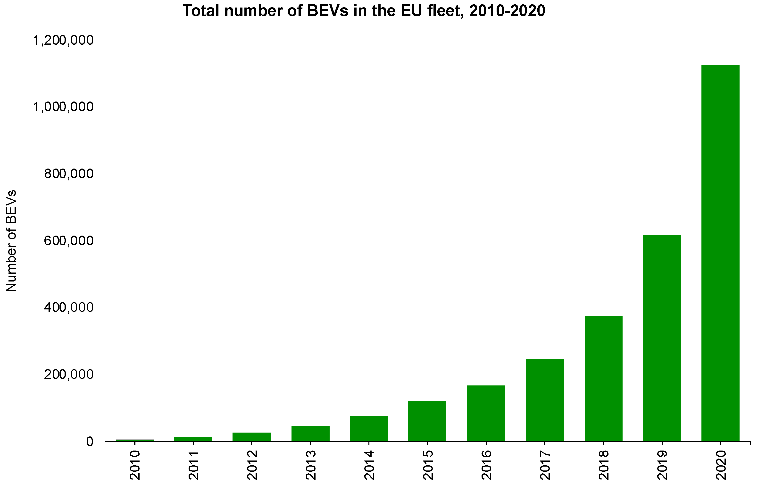
Indeed, when we addressed the total number of BEVs in the fleet, we can observe that in 2010, the EU had 5785 vehicles and in 2020 reached a value of 1,125,485 (see Figure 6 below).

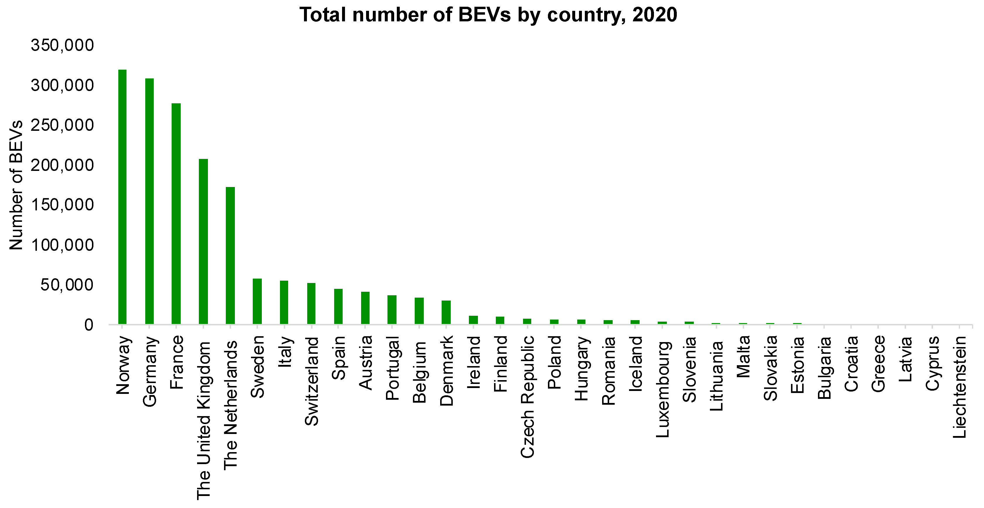
However, when we address the total number of BEVs in the fleet of each country of the European region in 2020, we can observe that Norway, Germany, France, the United Kingdom, and the Netherlands are the top five countries with a significant number of BEVs in the European Union. In contrast, Liechtenstein, Cyprus, and Latvia have fewer BEVs in the fleet (see Figure 7 below).

Moreover, in Norway, the number of BEVs in the fleet was 319,540 in 2020. In Germany, the number of BEVs in the fleet was 308,139. In France, the number of BEVs in the fleet was 277,001. In the United Kingdom, the number of BEVs in the fleet was 206,998. Moreover, in the Netherlands, the number of BEVs in the fleet was 172,534 in 2020. However, some countries in the European Union have a low number of BEVs in the fleet. For example, in Liechtenstein, the number of BEVs in the fleet was 222 in 2020. In Cyprus, this number was 251, while in Latvia, the number of BEVs in the fleet was 846.

Consequently, the increase in the number of BEVs in the EU’s fleet could have several implications for the energy demand, the economy, and the environment, as significantly documented in the literature (e.g., Hooftman et al. [16]; Bekel and Pauliuk [14]; Xu et al. [10]; Andersson and Börjesson [9]; Gryparis et al. [17]; and Burchart-Korol et al. [18]). Moreover, other non-EU countries have explored the BEVs performance, resulting in lower GHG emissions, such as China [19], Australia and New Zealand [20], and their benefits to developing countries in decarbonising the transport sector [21]. As we already know, there exist several drives that lead to the increase of GHGs emissions. Energy, economic growth, globalisation, urbanisation, trade, and transportation, are widely explored in literature (e.g., Squib and Benhmad [22]; Koengkan et al. [23]; Leitão [24]; Ouédraogo et al. [25]; Balsalobre–Lorente et al. [26]; Shahbaz et al. [27]; Simionescu [28]; Leitão et al. [29]; Nwani [30]; Uzuner et al. [31]; Dogan and Inglesi-Lotz [32]; Ike et al. [33]; Badulescu et al. [34]; Panait et al. [35]; Koengkan et al. [36]; Destek et al. [37]; and Grossman and Kruger [38,39]). Thus, the main objective of this investigation is to explore the effect of BEVs on GHGs emissions in the EU using a macroeconomic approach.

It is highlighted that no literature approaches the effect of BEVs on GHGs using a macroeconomic and econometric approach. Indeed, this topic of investigation has been linked and studied by science, namely by engineering. In this context, numerous studies in technologies and engineering demonstrate that electric vehicles improve the environment and reduce greenhouse effects assessing the life cycle of electric cars, with a particular focus on the hybrid electric vehicle, the plug-in hybrid electric vehicle, and the battery-electric vehicle (e.g., Andersson and Börjesson [9]; Zhao et al. [40]; Vilchez and Jochem [41]; Xiong et al. [42]; and Ajanovic and Haas [13]).

In light of this, we can conclude that there is a gap in economic theory about the impact of electric vehicles and their components, namely the batteries of electric cars, on GHG emissions. In other words, econometric models have not been using this variable or proxy to understand if electric vehicles and their components help with air quality, reduce GHGs emissions, and improve the environment. These models can show us that the economic models should be rethought in combination with different study objects. For example, the adoption of these models can contribute to the analysis of the relationship between economic growth, final energy consumption, and BEV adoption. Moreover, the introduction of this variable as an explanatory factor of the Kuznets environmental curve has not received due attention from economists what become one of the most relevant contributions of this work. Therefore, this investigation takes a vital role regarding the effect of BEVs on GHG emissions in the literature. This investigation is the first to use macroeconomic data and an econometric approach to identify this effect in the EU. Then, the main novelty of this work focuses on establishing a relationship between how BEVs interact with three variables: energy, economy, and environment, in European countries. Emphasising also that the methodology applied here can be reapplied in other countries, resulting in different results between this interaction.

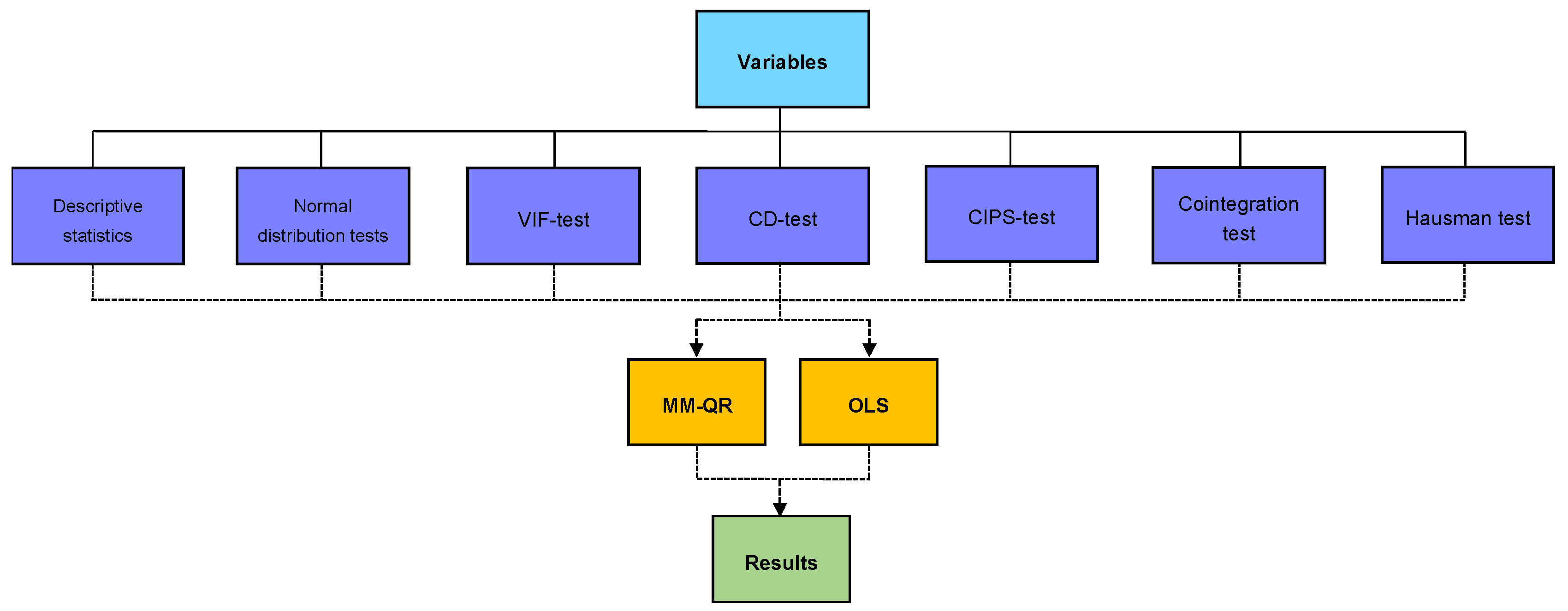
Well, faced with a lack of literature that approaches the effect of BEVs on GHG emissions in the European Union using a macroeconomic and econometric approach, we carry out the following question—Can battery-electric vehicles mitigate the greenhouse gas emissions in the European Union? This investigation will conduct an empirical analysis using macroeconomic panel data with twenty-nine countries, from the European Union, from 2010 to 2020, to answer this question. Therefore, this investigation will realise a macroeconomic analysis. For this research to be carried out, the method of moments quantile regression (MM-QR) and ordinary least squares (OLS) with fixed effects (to check the robustness of MM-QR’ results) will be used. The use of MM-QR accounts for the possibility that the environmental impacts of BEVs may be heterogeneous across the spectrum of the conditional distribution of GHG emissions in Europe. Thus, although BEVs can reduce GHG emissions, these advantages cannot be realised at the same level in all countries.

Furthermore, because the carbon intensity of the energy used to charge BEVs significantly impacts the potential benefit and varies between European countries, the potential benefit will vary. For example, adopting BEVs can significantly save in countries where renewable energy accounts for a considerable portion of the energy mix. However, in countries where fossil fuels account for a substantial portion of the energy mix, emissions from charging BEVs may not be offset during the driving phase. As a result, the environmental benefits for some countries are likely to be minor.

This empirical investigation will contribute to the literature, introducing a new analysis related to the effect of BEVs on GHGs in the European Union. This topic of investigation is not explored by economists and opens new opportunities to study the relationship between electric cars and environmental degradation using an econometric and macroeconomic approach. Moreover, this investigation will contribute with the introduction of econometric models (e.g., MM-QR and OLS with fixed effects) that is not explored by literature on this topic. Furthermore, this empirical investigation will help governments and policymakers develop more initiatives to promote electric cars in the EU and policies to reduce the consumption of non-renewable energy sources, energy efficiency, and environmental degradation. Finally, this research topic can open a channel of policy discussion between industry, government, and researchers, as a crucial step towards ensuring that BEVs provide a climate change mitigation pathway in the region.

The remainder of this paper is divided into sections: a literature review in Section 2, data presentation and study methodology in Section 3, empirical results in Section 4, discussions of results in Section 5, conclusions and policy implications in Section 6, and limitations of the study in Section 7.

2. Literature Review

This section presents recent literature explaining the relationships between economic growth, non-renewable energy consumption, electric vehicles, and carbon dioxide emissions.

2.1. The Causality between Economic Growth and Carbon Dioxide Emissions

The links between economic growth and carbon dioxide emissions have been studied frequently by economists, especially since the 1990s with the overview of the environmental Kuznets curve [38,39]. In general, empirical studies find a U–shaped relationship between economic growth and polluting emissions. In the first stage of pre-industrialisation, countries are not aware of environmental issues, showing that economic growth is associated with high pollution levels. In the next step, in a phase of industrialisation, countries tend to reduce pollution emissions because they are aware of the environmental problems. This assumption is considered valid by the literature review.

More recently, new variables were introduced in the literature. Globalisation, renewable energies, corruption, economic complexity, urbanisation, tourism, democracy, and public health were introduced in the environmental Kuznets curve to assess their impact on air quality (e.g., Koengkan et al. [23]; Leitão [24]; Balsalobre–Lorente et al. [26]; Leitão et al. [29]; Nwani [30]; Uzuner et al. [31]; and Ike et al. [33]). Considering the presence of structural breaks for European Union countries, the empirical study of Ketenci [43] concluded that there are no found assumptions of EKC for the period 1974–1989, except for Sweden. Nevertheless, the EKC is valid for France, Germany, Greece, Italy, and Portugal when the author considers from 1960 to 2015 [43]. In this line, Panait et al. [35] studied EKC for EU countries between 1960 and 2014. The results showed that exports negatively affect pollution emissions, and imports positively impact CO₂ emissions. However, the authors do not find the expected signs for the correlation between income per capita, squared income per capita, and CO₂ emissions, i.e., according to their results, the variables of income per capita and squared income per capita present an opposite expected sign.

Recently, the ecological footprint was examined using the environmental Kuznets curve by Squib and Benhmad [22]. The authors used as sample 22 European countries, and their study validates the nonlinear relationship between economic growth and ecological footprint. Furthermore, they found that energy consumption encourages an environmental footprint. Similarly, the empirical research of Badulescu et al. [34] found EKC assumptions for EU countries.

Simionescu [28] tested the EKC for six Central and Eastern European countries, and the econometric results demonstrated a nonlinear relationship between renewable energy and carbon dioxide emissions. Besides, the relationship between economic growth and CO₂ emissions found an inverted N-shaped curve.

Then, the literature review applied to the EU countries is inconclusive regarding the environmental Kuznets curve. However, most empirical studies support a positive relationship between economic growth and climate change, showing a linear relationship between economic growth and carbon dioxide emission. Furthermore, there is a bidirectional relationship between growth and carbon dioxide emissions.

2.2. The Relationship between Energy Consumption and Carbon Dioxide Emissions

As in the previous relationship, the impact of non-renewable energy consumption is relatively abundant in the literature. Therefore, this item will try to present a non-exhaustive survey that justifies the introduction of energy consumption in the Kuznets environmental equation. Thus, as a rule, empirical studies find a positive association between energy consumption and carbon dioxide emissions, demonstrating that the intensity of non-renewable energy causes environmental damage. Indeed, it stimulates the climate change since this variable is associated with activity economy (e.g., Dogan and Inglesi-Lotz [32]; Ouédraogo et al. [25]; Shahbaz et al. [27]; Koengkan et al. [36]; and Destek et al. [37]). It is, thus, possible to observe a bidirectional relationship between the two variables when studies apply Granger causality or the more recent Dumitrescu and Hurlin technique.

The empirical study of Dogan and Inglesi-Lotz [32] evaluated the experience of European countries, and they found a nonlinear relationship between economic growth and pollution emissions. The variable of industry value-added also presents an inverted U curve. Moreover, the variables of energy structure, energy intensity, and population positively affect carbon emission, showing environmental damage. Similarly, Sharma et al. [44] evaluated the impact of energy consumption on the association between per capita income and CO₂ emissions and financial development and CO₂ emissions from 1976 to 2015, in Asian countries. The authors confirm that energy consumption leads to environmental pollution at the lower level of income; on the other hand, the impact of carbon emissions becomes weak at the higher level of income.

The environmental Kuznets curve applied to 11 African countries was investigated by Ouédraogo et al. [25]. Considering the causality results using Dumitrescu and Hurlin methodology, this empirical study showed bidirectional causality between CO₂ emission and economic growth. The same is valid for the relationship between carbon dioxide emissions and energy consumption and bidirectional causality between economic growth and energy use. Ardakani and Seyedaliakbar [45] investigated the relation between CO₂ emission, energy consumption, and GDP through multivariate linear regression in seven oil-rich countries in the MENA region to assess whether the environmental Kuznets curve can be confirmed or not. The authors confirmed EKC only in three countries (Oman, Qatar, and Saudi Arabia).

For instance, Shahbaz et al. [27] considered India’s experience and tested the sustainable development goals considering a NADRL model (nonlinear autoregressive distributed lag). They concluded that India needs improvements in environmental aspects to obtain sustainable development because economic growth depends on non-renewable energy and imported crude oil.

The linkage between economic growth, energy, and carbon dioxide emissions applied to four Andean countries was investigated by Koengkan et al. [36]. They found bidirectional causality between growth and energy using an autoregressive panel regression. Thus, the economic activity needs energy intensity levels directly associated with energy demand theory. Moreover, the authors also found bidirectional causality between carbon dioxide emissions and economic growth. Therefore, energy consumption is directly related to environmental degradation.

Subsequently, Destek et al. [37] evaluated the EKC hypothesis using a dependent variable ecological footprint, considering 1980–2013. The authors used panel cointegration (FMOLS fully modified ordinary least squares) and DOLS (dynamic ordinary least squares). The results demonstrated that economic growth presents an inverted U-shaped ecological footprint. Furthermore, non-renewable energy positively affects the environmental footprint, and renewable energy and trade improve the environment.

2.3. The Link between Electric Vehicles and Carbon Dioxide Emissions

The transport sector, namely parts and components, contributes to the fragmentation or outsourcing process of the international economy [46], where vertical product differentiation predominates. On the other hand, the tertiarization of bilateral trade leads to economic growth. Besides, trade intensity and intra-industry trade reduce carbon dioxide emissions and climate change [47,48].

The transport sector’s impact on carbon dioxide emissions and its relationship with the Kuznets environmental curve has been the object of study [49,50]. The study proposed by Ferreira et al. [49] applied to the case study for the BRICS countries (Brazil–Russia–India–China, and South Africa), using panel data for the transport sector, demonstrates that gas consumption and oil consumption have a positive effect on dioxide emissions of carbon.

The Malaysian experience was investigated by Go et al. [50] using the FMOLS (fully modified ordinary least squares), CCR (canonical cointegration regression), and DOLS (dynamic ordinary least squares) estimators. The authors used as dependent variable carbon dioxide emissions from the transport sector and as independent variables income per capita squared income per capita, corruption and oil consumption. The econometric results show that carbon dioxide emissions tend to increase with bribery and the assumptions of the environmental curve applied to the transport sector are not valid.

For the analysis of the eight leading countries in the global electric vehicle market (i.e., China, France, Germany, India, Japan, the Netherlands, Norway, and the UK), Xu et al. [51] used monthly data from 2009 to 2017, investigating the dynamic linkages between the stock of electric vehicles and carbon dioxide emissions. The authors used the quantile-on-quantile regression approach and obtained heterogeneous results between countries. However, overall, they find that electric vehicles negatively affect carbon dioxide emissions, and carbon dioxide emissions weakly and positively affect electric vehicles. Thus, there is a mixed directionality of causality between the two variables.

However, a meta-analysis on the relationship between electric vehicles and carbon dioxide emissions allows us to conclude that there is a gap in economic theory about the impact of electric cars and their components, namely the batteries of electric vehicles, on carbon dioxide emissions. In other words, econometric models have not been using this variable or proxy to understand if electric cars and their components help with air quality, reduce carbon dioxide emissions, and improve the environment. Indeed, very few studies have used econometric methods to explore the relation between electric vehicles and carbon emissions [51]. The introduction of this variable as an explanatory factor of the Kuznets environmental curve has not received due attention from economists. Still, as mentioned, there is an intuition that the batteries of electric vehicles can improve ecological issues. Intuitively we consider that electric cars improve and reduce climate change. This premise has been linked and studied by science, namely by engineering. In this context, numerous studies in technologies and engineering demonstrate that electric vehicles improve the environment and reduce greenhouse effects assessing the life cycle of electric cars, with a particular focus on the hybrid electric vehicle, the plug-in hybrid electric vehicle, and the battery-electric vehicle (e.g., Andersson and Börjesson [9]; Zhao et al. [40]; Vilchez and Jochem, [41]; Xiong et al. [42]; Ajanovic and Haas [13]).

The article by Ajanovic and Haas [13] draws some interesting conclusions, considering that electric vehicles contribute to the improvement of the environment, but emissions depend on the vehicle’s production and use. Furthermore, the authors conclude that the environmental benefits depend on the use of renewable electricity. The study by Zhao et al. [40] looks at the impact of plug-in hybrid electric vehicles (PHEV) on the environment, concluding that the use of PHEV allows for a more sustainable environment, using tall batteries and, whenever necessary, replacing these batteries. In this line, Andersson and Börjesson [9] concluded that renewable fuels tend to reduce greenhouse effects in hybrid electric vehicles, plug-in hybrid electric vehicles, and battery-electric vehicles. Nevertheless, regardless of the use of renewable electricity, it is also essential to highlight the increase in the efficiency of electric vehicles. Considering different driving conditions, empirical data from Germany shows that battery-electric vehicles consume on average 67% less energy than internal combustion vehicles [52]. Indeed, technological innovation positively impacts energy efficiency [53].

The construction of explanatory scenarios for China, France, Germany, India, Japan, and the United States using electric cars was developed by Vilchez and Jochem [41]. The results show that electric vehicles can reduce greenhouse effects; however, the production must use clean energies.

A comparison between electric vehicle batteries (BEVs) and plug-in hybrid electric vehicle batteries (PHEVs) was proposed by Xiong et al. [42] for the Chinese case. In this study, the authors assess the greenhouse effects on the environment when comparing these types of vehicles. Like previous studies, the results showed that electric vehicle batteries (BEVs) decrease greenhouse effects and energy consumption.

The following section will be presented the data and method used to accomplish this empirical investigation.

3. Data and Method

This section will be divided into two parts. The first will approach the group of countries and data/variables used in this investigation, while the second will show the method.

3.1. Data and Hypotheses

This investigation uses annual data that was collected from 2010 to 2020, to twenty-nine European countries (e.g., Austria, Belgium, Bulgaria, Croatia, Cyprus, Czechia, Denmark, Estonia, Finland, France, Germany, Greece, Hungary, Iceland, Ireland, Italy, Latvia, Lithuania, Luxembourg, Norway, Netherlands, Poland, Portugal, Romania, Slovakia, Slovenia, Spain, Sweden, and the United Kingdom). This group of countries was selected because the BEVs gradually penetrated the European Union (EU) market. The region has registered an increase in new electric car registrations annually, from 700 units in 2010 to about 550,000 units in 2019. Nevertheless, they still account for a market share of only (3.5%) of newly registered passenger vehicles [15]. Moreover, as we are addressing a macroeconomic aspect, it is convenient to use all countries from the EU. Unfortunately, the European Alternative Fuels Observatory (EAFO) provides data from 2010 until 2020. The variables that were chosen to perform this investigation will be shown in

Table 1. Variables’ description and descriptive statistics.

Dependent Variables
Variable	Description		Time	Source
GHGs	Greenhouse gas emissions per capita. This indicator includes carbon dioxide (CO2), methane (CH4), nitrous oxide (N2O), and the so-called F-gases (hydrofluorocarbons, perfluorocarbons, nitrogen trifluoride (NF3), and sulphur hexafluoride (SF6).		2010–2020	Eurostat [54]
Independent variables
GDP	GDP per capita based on purchasing power parity (PPP). This variable is converted to international dollars using purchasing power parity rates.		2010–2020	World Bank Open Database [55]
ENERGY	Final energy consumption in thousand tonnes of oil equivalent per capita. Final energy consumption covers the energy consumption of end-users, such as industry, transport, households, services, and agriculture.		2010–2020	Eurostat [56]
BEVs	The number of battery electric vehicles (BEVs) registered in the fleet.		2010–2020	European Alternative Fuels Observatory (EAFO) [15]
Variables	Descriptive Statistics
	Obs.	Mean	Std.-Dev.	Min.
LnGHGs	280	2.2281	0.3398	1.6486
LnGDP	290	10.5781	0.3738	9.7665
LnENERGY	290	3.9564	0.4332	2.1972
LnBEVs	290	5.1711	2.8874	0.0000

Notes: (Ln) denotes variables in the natural logarithms; Obs. denotes the number of observations in the model; Std.-Dev. denotes the Standard Deviation; Min. and Max. denote Minimum and Maximum, respectively; the command sum of Stata was used.

below.

Next, we present the hypotheses formulated considering the literature review shown in this investigation.

Hypothesis 1 (H1).

The development of economic activity and economic growth presuppose high levels of carbon dioxide emissions.

Considering the Kuznets environmental curve arguments, empirical studies usually find a positive association between economic growth and pollution emissions. In this context, Badulescu et al. [34], Panait et al. [35], Squib and Benhmad [22], and Simionescu [28] support the formulated hypothesis.

Hypothesis 2 (H2).

Non-renewable energies and their energy intensity stimulate greenhouse effects.

Several studies such as Destek et al. [37], Koengkan et al. [36], Sharma et al. [44], Ardakani and Seyedaliakbar [43] found a statistically significant positive correlation between energy consumption and carbon dioxide emissions.

Hypothesis 3 was constructed based on empirical studies between the association of electric vehicles batteries and carbon dioxide emissions. However, as mentioned in the review from the literature and after having carried out a meta-analysis on the association of electric vehicle batteries and pollution levels, we observed that in economics science, there is little empirical evidence as far as we know. However, some studies, such as Andersson and Börjesson [9]; Zhao et al. [40]; Vilchez and Jochem, [41]; Xiong et al. [42]; Ajanovic and Haas [13], from the engineering areas allowed us to formulate the following hypothesis:

Hypothesis 3 (H3).

Electric vehicle batteries reduce climate change and improve air quality.

In this context, the investigation will use the following variables GHGs, GDP, ENERGY, and BEVs. The variable GHGs is our dependent variable, while GPD, ENERGY, and BEVs are our independent variables. Moreover, the variables GDP and ENERGY are the control variables of our empirical model. Furthermore, it is worth remembering that the literature windily uses the variable GHGs as a dependent variable. The same occurs with the variables GDP and ENERGY, which also are windily used by literature as an independent variable to explain the increase of GHGs. However, only the variable BEVs was not approached by literature to explain the rise of GHGs in a macroeconomic and econometric context. At last, the variables in per capita values such as GHGs, GDP, and ENERGY were used to reduce the effects of population disparity. Therefore, after presenting the variables, it is also necessary to present the method used.

Then we present some theoretical foundations about the independent variables under study and carbon dioxide emissions.

Theoretically, the greenhouse gas emission–income nexus suggests that economic growth increases greenhouse gas emissions. This effect is due to the high consumption of energies intensive in carbon in countries’ first stages of industrialisation [53]. This phenomenon leads to an inverted U-shaped EKC. In this line, the expected sign of the coefficient for economic growth is positive. Moreover, higher energy consumption leads to an increase in greenhouse gas emissions [27]. Thus, we expect the association between energy consumption and greenhouse gas emission to be positive. The current study is synthesised from the energy–growth–environmental degradation literature. However, incorporating the battery-electric vehicle variable into our empirical model distinguishes it from existing studies in the literature. The battery-electric vehicles are expected to increase environmental quality by mitigating greenhouse-gas emissions [42]. This study extends the EKC framework by using the functional relationship based on the growth-induced environmental degradation hypothesis with the inclusion of battery-electric vehicles to investigate the relationship between the variables mentioned above.

3.2. Method

This subsection presents the main methods used in this empirical investigation and the preliminary tests necessary to carry out.

3.2.1. Method of Moments Quantile Regression (MM-QR)

The recent and novel Method of Moments Quantile Regression (MM-QR) approach for panel fixed effects developed by Machado and Silva [57] is adopted to explore the impact of battery electric vehicles on greenhouse gas emissions for a panel of 28 OECD countries. Furthermore, unlike previous panel quantile regressions proposed by Canay [58], Lamarche [59], and Koenker [60] used the MM-QR with fixed effects technique. This approach captures the unobserved distributional heterogeneity across countries within a panel. Another merit of the MM-QR is that it assumes that covariate only affects the variable of interest through the channel of location and scale functions relative to a mere shifting location [61]. Thus, it is possible to investigate the conditional heterogenous covariance effects of the determinants of greenhouse gas emissions at different quantiles of its distribution for the countries under consideration.

Following the study of Machado and Silva [57], using data highlighted variables under review $\{{(GHG{s}_{it},X_{it}^{\prime })}^{\prime }\}$ from a bloc of $n$ countries $i=1,2,\dots ,n$ overtime periods $t=1, 2,\dots ,T$, we conduct a location-scale model of the conditional quantiles $Q_{GHG}\left(\tau |X_{it}\right)$ as given (see Equation (1) below).

$$GHG{s}_{it}={\alpha }_i+X_{it}^{\prime }\beta +\left(i+Z_{it}^{\prime }\gamma \right)U_{it}$$

(1)

with Pr$\left\{{\delta }_i+Z_{it}^{\prime }\gamma >0\right\}=1$ and the unknown parameters (${\alpha }_i, {\delta }_i),$| $i=1,2,\dots ,n$ measure the fixed effect for individual and $Z$ is a known differentiable (with Pr = 1) transformation of the elements of X. $U_{it}$ is the error term which is independently and identically distributed across $i$ and $t$, uncorrelated with $X_{it}$. Model (1) can be extended. See Equation (2) below.

$$Q_{GHG}\left(\tau |X_{it}\right)=\left({\alpha }_i+{\delta }_{i}q\left(\tau \right)\right)+X_{it}^{\prime }\beta +Z_{it}^{\prime }\gamma q\left(\tau \right)$$

(2)

where the scalar coefficient ${\alpha }_i\left(\tau \right)={\alpha }_i+{\delta }_{i}q\left(\tau \right)$ denotes the quantile- $\tau$ fixed effect for an individual country. The distributional impact varies from the classical fixed effect, given that it is not location fixed. To this end, the distributional effect depicts the time-invariant traits that allow for other variables to have diverse effects on investigated countries (For the sake of brevity, see Machado and Silva [57] for more insight on the Method of the Moments Quantile Regression approach for panel fixed effects).

3.2.2. Ordinary Least Squares (OLS) with Fixed Effects

The OLS estimates the slope and intercepts for a set of observations and other estimates of mean response for the fixed predictors using the conditional mean function in this study (see Equation (3), below).

LnGHGs_it = β₀ + β₁LnGDP_it + β₂LnENERGY_it + β₃LnBEVs_it + ε_it

(3)

where β₀ is the intercept, and β is the value of fixed covariates being fitted to predict the dependent variable LnGHGs_it, ε_i is the error term, and each variable enters regression for country i at year t. Thus, OLS modelling allows to describe the relationship between the covariates but cannot be extended to non-central locations in the case of shapeshifts. OLS is also heavily influenced by outliers [62,63].

Indeed, before realising the MM-QR and OLS with fixed effects, we must realise the preliminary tests. Therefore, we will evidence the preliminary tests used in this empirical investigation.

3.2.3. Preliminary Tests

As mentioned before, preliminary tests are necessary before the model estimations. Indeed, these tests are necessary to detect the proprieties of variables used in this empirical study and verify the existence of singularities, which is not considered and could lead to inconsistent and incorrect interpretations. To this end, some preliminary tests will be applied in the study, as shown in

Table 2. Preliminary tests.

Test	Reference	Description
Shapiro-Wilk	Shapiro and Wilk [64]	It checks the normality of the panel model.
Skewness/Kurtosis	D’Agostino et al. [65]	Based on combining Skewness and Kurtosis amounts, it checks the normality.
Variance Inflation Factor (VIF)	Belsley et al. [66]	It measures multicollinearity in a regression analysis.
Cross-sectional dependence (CD)	Pesaran [67]	It recognises the presence of cross-sectional dependence in the model.
Panel Unit Root test (CIPS)	Pesaran [68]	It detects the presence of unit roots.
Westerlund panel cointegration	Westerlund [69]	It checks whether cointegration exists or not by determining whether error correction is present for individual model members and the panel as a whole.
Hausman	Hausman [70]	It verifies the random effects vs fixed effects; Identifies heterogeneity.

Notes: This table was created by the authors.

below.

Then, this investigation will follow the following conceptual framework (see Figure 8), highlighting the methodological approach.

The empirical analysis was carried out using the econometric software Stata 17.0. Moreover, this investigation will use the following Stata commands (e.g., sum, sktest, swilk, vif, xtcd, multipurt, xtwest, hausman, xtqreg, and xtreg). The next section will present the empirical results of this investigation.

4. Empirical Results

As mentioned before, this section is devoted to the empirical results of this study, which starts with the preliminary tests and then represents the model estimation results. The descriptive statistics of the variables were presented in the previous section. Next, the normality test was conducted to identify the distribution of the variables, which includes the Skewness/Kurtosis tests [65] and Shapiro–Wilk tests [64].

Table 3. Normal distribution tests.

Variables	Obs.	Skewness	Kurtosis	Skewness/Kurtosis Tests	Shapiro-Wilk Test
				Prob > Chi2	Prob > z
LnGHGs	280	0.0003	0.8847	0.0034 **	0.0000 ***
LnGDP	290	0.0034	0.2217	0.0100 **	0.0000 ***
LnENERGY	290	0.0000	0.0016	0.0000 ***	0.0000 ***
LnBEVs	290	0.3782	0.0008	0.0048 **	0.0002 ***

Notes: ***, **, denote statistically significant at (1%), and (5%) level; (Ln) denotes variables in the natural logarithms; the commands sktest and swilk of Stata were used.

below shows the results from the normal distribution tests.

The results of the normal distribution tests revealed that LnBEVs is highly skewed. In addition, the combined skewness–kurtosis test proposed by D’Agostino et al. [65] showed that the null hypothesis of the normal distribution could be rejected for the data from this group of countries during this specific period. Moreover, testing normality applying the Shapiro–Wilk test, the null hypothesis of normal distribution for all variables in the model can be rejected; hence, all model variables are not normally distributed.

In the next step, it is essential to test and measure multicollinearity between variables in the model; therefore, the variance inflation factor (VIF) test [66] was calculated.

Table 4. VIF-test.

Variables	VIF	1/VIF	Mean VIF
LnGHGs
LnGDP	2.88	0.3466	2.19
LnENERGY	2.28	0.4385
LnBEVs	1.41	0.7081

Notes: (Ln) denotes variables in the natural logarithms; the command vif of Stata was used.

shows the model’s VIF-test result. The mean VIF of 2.19 represents low multicollinearity among the model variables, as the rule of thumb suggests a mean VIF value of 6 or lower to proceed with the model estimation [71].

Applying the Pesaran CD-test developed by Pesaran [67] to identify the presence of cross-sectional dependence (CSD) in the panel data (

Table 5. Pesaran CD-test.

Variables	CD-Test	p-Value
LnGHGs	19.69	0.000 ***
LnGDP	49.15	0.000 ***
LnENEGY	54.45	0.000 ***
LnBEVs	54.45	0.000 ***

Notes: *** denotes statistically significant at (1%) level; (Ln) denotes variables in the natural logarithms; the command xtcd of Stata was used.

) shows the existence of cross-section dependence in all variables of the model. Furthermore, this test indicates that the countries selected in this study represent the same characteristics and shocks [23].

Verifying the order of integration of the variables in the model is essential in deciding whether to proceed with the cointegration test. Hence, the panel unit root tests were applied, such as the CIPS-test developed by Pesaran [68].

Table 6. Unit Root test.

Variables	Panel Unit Root Test (CIPS) (Zt-Bar)
	Without Trend		With Trend
	Lags	Adjusted t	Adjusted t
LnGHGs	1	−1.210	−2.516 ***
LnGDP	1	−3.900 ***	−3.158 ***
LnENERGY	1	−0.143 **	−3.296 ***
LnBEVs	1	−1.009	−1.661 **

Notes: ***, ** denote statistically significant at (1%) and (5%) levels; (Ln) denotes variables in the natural logarithms; the command multipurt of Stata was used.

below shows the results from the unit root tests. For example, the panel unit root test (CIPS) indicates that the variables LnGDP and LnENERGY without and with the trend are stationary or I(1). On the contrary, the variables LnGHGs and LnBEVs, without and with the trend, are between the I(0) and I(1) order of integration.

The existence of I(1) variables in the model suggests the necessity of verifying the presence of cointegration between these variables. In doing so, the Westerlund panel cointegration test [69] is applied in this study.

Table 7. Westerlund panel cointegration test.

Variables LnGDP and LnENERGY
Statistic	Value	Z-Value	p-Value
Gt	0.216	11.951	1.000
Ga	0.427	7.488	1.000
Pt	1.156	9.004	1.000
Pa	0.490	5.726	1.000

Notes: The command xtwest with option constant of Stata was used. H₀: No cointegration; H₁ Gt and Ga test the cointegration for each country individually, and Pt and Pa test the cointegration of the panel.

below represents the Westerlund panel cointegration test results. This test is for checking the presence of cointegration between LnGDP and LnENERGY.

The results of the Westerlund panel cointegration tests revealed that the null hypothesis of no cointegration could not be rejected. All panel statistics, such as Gt and Ga, test cointegration for each country individually, and Pt and Pa that test the cointegration of the panel also do not reject the null hypothesis. The Hausman test compares the model’s random effects (RE) and fixed effects (FE). The null hypothesis of this test suggests that the difference in coefficients is not systematic, where the random effects are the most suitable estimator [23]. The results of this test are presented in

Table 8. Hausman test.

Dependent variable LnGHGs
Variables	(b) Fixed	(B) Random	(b-B) Difference	Sqrt(diag(V_b-V-B)) S.E.
LnGDP	−0.0961	−0.0536	−0.0424	0.0136
LnENERGY	0.8986	0.7997	0.0989	0.0278
LnBEVs	−0.0123	−0.0138	0.0014	0.0004
Chi2 (3)	15.73 ***

Notes: *** denotes statistically significant at the (1%) level; (Ln) denote variables in natural logarithms; the Stata command hausman (with the options, sigmaless) was used.

below, which indicates that the null hypothesis cannot be accepted, confirming the presence of fixed effects in the model.

The model can be estimated with the quantile regression and the OLS model with fixed effects at the final stage.

Table 9. Estimation results from Quantile regression and OLS with fixed effects.

Independent Variables	Dependent Variable (LnGHGs)
	Quantiles			OLS
	25th	50th	75th	Fixed Effects
LnGDP	0.6948 ***	0.6516 ***	0.4148 ***	−0.0961 *
LnENERGY	0.1665	0.2178 ***	0.2323 ***	0.8986 ***
LnBEVs	−0.0339 ***	−0.0490 ***	−0.0348 ***	−0.0123 ***
Constant	−4.1859 **	−3.2541 ***	−0.5458	8.1558 ***
Obs	280	280	280	280
Pseudo R2	0.3087	0.3526	0.3506	0.3705

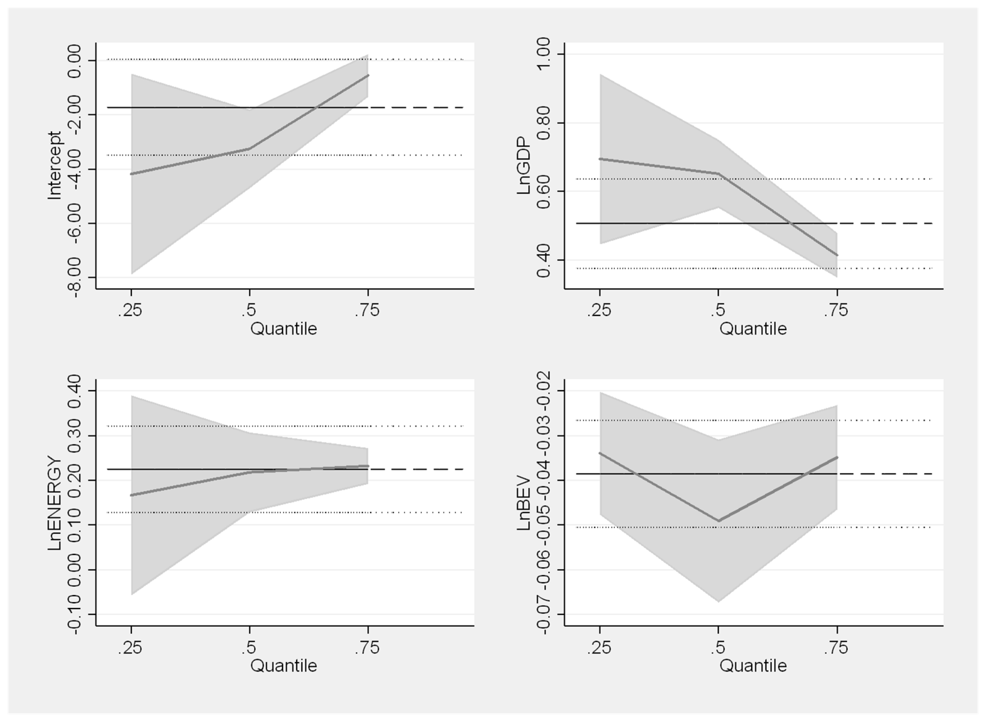
Notes: ***, **, * denote statistically significant at (1%), (5%), and (10%) levels; (Ln) denotes variables in the natural logarithms; the command xtqreg with option reps (350) and xtreg with option fe of Stata was used.

represents the results of quantile regression and OLS with fixed effects of the model. Estimating the model with the quantile regression indicates that in all three quantiles, the variable LnGDP causes a positive impact on LnGHGs. This variable is statistically significant at a (1%) level with quantile regression. According to previous studies (e.g., Koengkan et al. [23]; Nwani [30]; and Uzuner et al. [31]), this result shows that economic activity is direct with environmental damage and climate change.

In the 50th and 75th quantiles, the variable LnENERGY also causes a positive effect on the dependent variable, and the variable is statistically significant at a (1%) level. Hence, both economic development and energy consumption increase the emissions of GHGs in EU countries. However, the variable LnBEVs in the 25th, 50th, and 75th quantiles result in a negative impact on the variable LnGHGs, meaning that the battery electric vehicles are capable of mitigating GHGs emissions. Our results are according to the conclusions of engineering studies. Thus, as concluded by Andersson and Börjesson [9], Zhao et al. [40], electric batteries aim to reduce CO₂ emissions.

Moreover, the estimation results applying the OLS model with fixed effects indicated that the variable LnGDP has a negative impact on the variable LnGHGs; therefore, it is possible to conclude that economic development mitigates the emissions of GHGs. This finding contradicts the results from the quantile regression. The variable LnENERGY causes a positive impact on the variable LnGHGs, indicating that energy consumption contributes to an increase in GHGs emissions. In contrast, the variable LnBEVs causes negative effects, which are in line with the results from the quantile regression. This result indicates that BEVs are capable of mitigating the emissions of GHGs.

Figure 9 illustrates the graphical results of the quantile regression. The shaded areas are (95%) confidence bands for the quantile regression estimations. The vertical axis represents the elasticities of the explanatory variables. The horizontal lines depict the conventional (95%) confidence intervals for the OLS coefficients.

Moreover, Figure 10 below summarises the impact of independent variables on dependent ones. This figure was based on results from Table 9.

This section approached the empirical results, starting with the preliminary tests, and presenting the main model regression results. The following section will present the discussions and presented the possible explanations for the results that were found.

5. Discussions

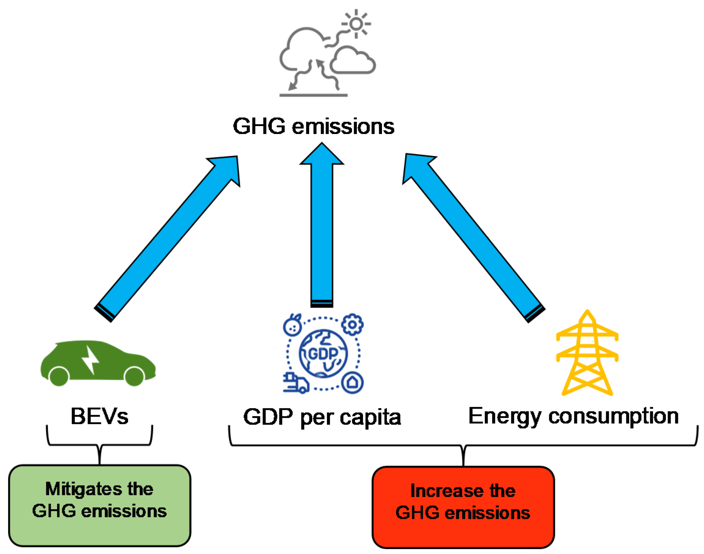
In this section, we will address the discussions of results that were found in this empirical investigation. As shown in Section 4, the economic growth and the final energy consumption increase the GHG emissions, while the BEVs mitigate them. In light of this finding, we arose the following questions: What are the possible explanations for the results found? Are these results in accordance with the literature? The positive impact of economic growth on GHG emissions in the European region was confirmed by several authors in the literature (e.g., Mendonça et al. [72]; Nawaz et al. [73]). For example, Mendonça et al. [72] studied the impact of GDP, population, and renewable energy generation in CO₂ emissions in 50 countries (including the EU countries) for the period between 1990 and 2015. The authors found that an increase of (1%) in the GDP generates (0.27%) in CO₂ emissions in all study countries. According to the authors, this result was found because most study countries depend on energy from fossil fuels to grow.

This vision is shared by Nawaz et al. [73]. According to the authors, modern production techniques make industrial production more attractive and effective in developing and advanced nations. Consequently, it increases the utilisation of non-renewable energy sources. Indeed, this increase substantially influences per capita GDP and improves the quality of life by increasing the provision of goods. Indeed, the efforts to increase per capita GDP through increasing production impact negatively the environment.

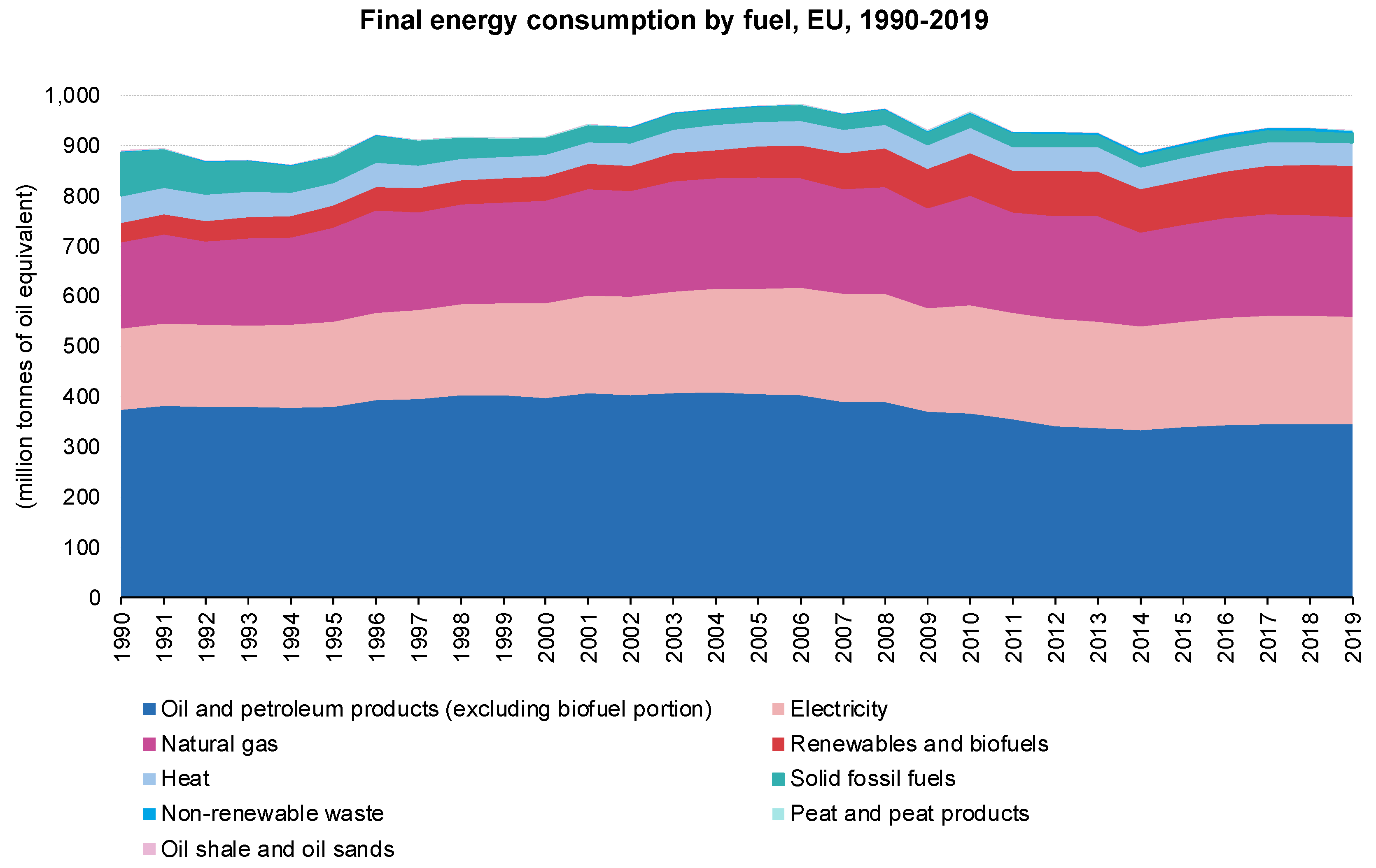
Indeed, the evidence that European countries depend on non-renewable energy to grow, as mentioned by Mendonça et al. [72], makes perfect sense. For example, in 1990, (71%) of the final energy consumption came from non-renewable energy sources, while renewable energy sources had a share of (4.33%) in the energy mix in the European region. However, in 2019, this scenario changed, where fossil fuels had a share of (69.4%) in the energy mix, while renewable energy had a share of (15.8%) (see Figure 11 below).

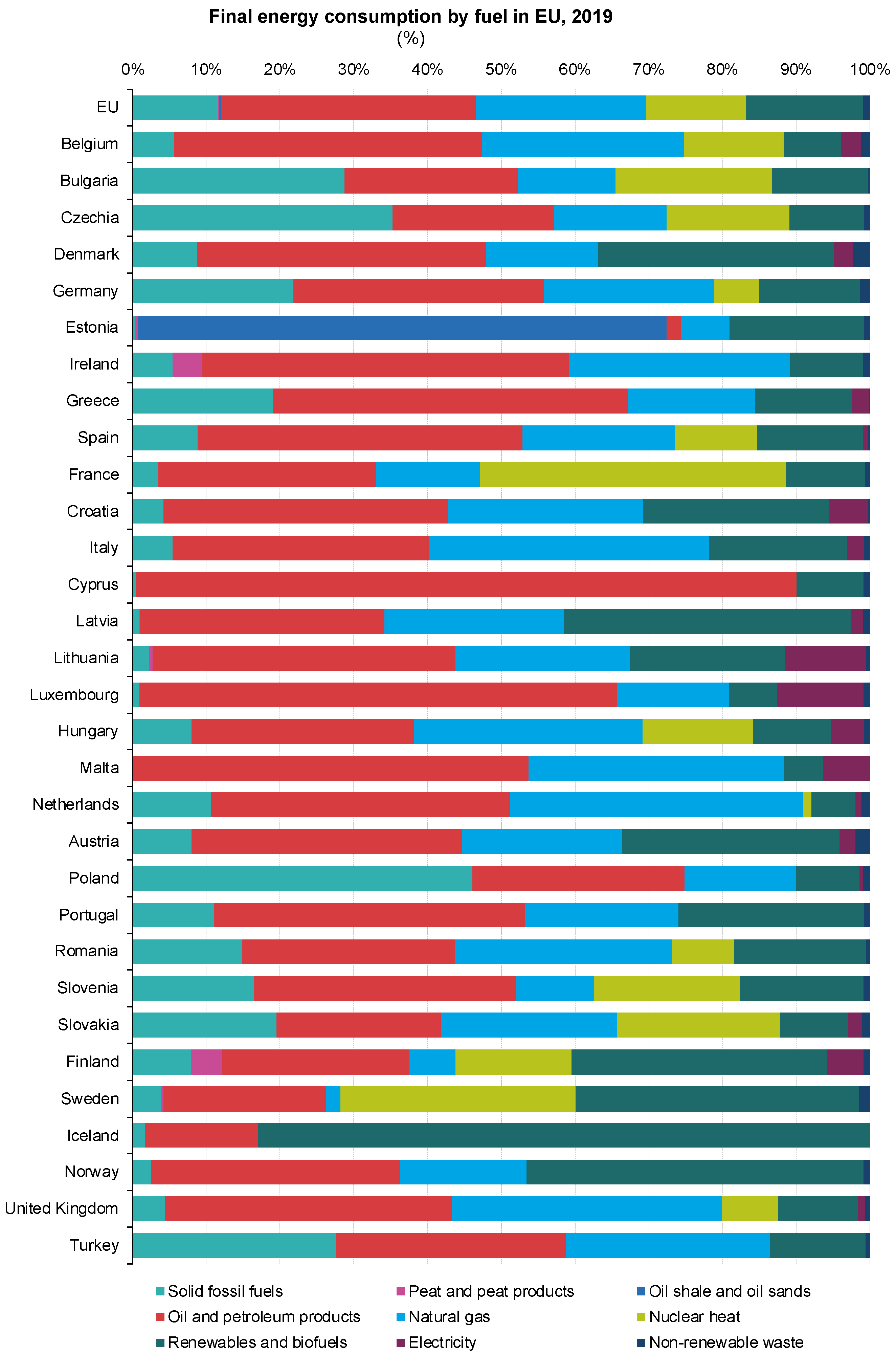
However, the mix of fuels and their share in final energy consumption varies in different EU countries due to the natural resources available, the industry in each country, and national resources in energy systems. Thus, for example, we can include the share of solid fossil fuels, crude oil, petroleum products, and natural gas in final energy consumption below (50%) (e.g., Estonia (9.1%); Sweden (28.7%); Finland (39.4%); and France (48.25%)) (see Figure 12 below).

Moreover, it should be noted in the figure above, France and Sweden were also the countries with the highest contribution of nuclear heat to the final energy consumption, where both countries contributed with (42.3%) and (32.8%), respectively. In Sweden and Latvia, renewable energies accounted for just short of (40%) of their final energy consumption in 2019 (39.6% and 38.9%, respectively), with Finland closely following at (34.6%). The lowest participation of renewable energy was registered in Malta (5.4%), the Netherlands (6.0%), and Luxembourg (6.5%).

Therefore, the capacity of energy consumption to increase GHG emissions in the European countries is associated with economic activity, as mentioned above. Several authors found this evidence (e.g., Ouédraogo et al. [25]; Shahbaz et al. [27]; Mendonça et al. [72]; Dogan and Inglesi-Lotz [32]; Nawaz et al. [73]; Koengkan et al. [36]; and Destek et al. [37]). Indeed, the increase in economic activity leads to increased energy consumption from non-renewable energy sources. Moreover, the evidence that economic growth increases the final energy consumption in the European countries was found by us (see

Table 10. Estimation results from Quantile regression and OLS with fixed effects.

Independent Variables	Dependent Variable (LnENERGY)
	Quantiles			OLS
	25th	50th	75th	Fixed Effects
LnGDP	0.8047 ***	0.9423 ***	1.0445 ***	0.4667 ***
LnBEV	−0.0034	−0.0264 ***	−0.0341 ***	−0.0154 ***
Constant	−14.0654 ***	−15.2045 ***	−16.1439 ***	−10.2377 ***
Obs	290	290	290	290
Pseudo R2	0.3208	0.3995	0.4618	0.5827

Notes: *** denotes statistically significant at (1%) level; (Ln) denotes variables in the natural logarithms; the command xtqreg with option reps (350) and xtreg, fe of Stata were used.

below).

Therefore, as shown in Table 10 above, in the quantile model regression, the economic growth in 25th, 50th, and 75th quantiles increase the final energy consumption, while the BEVs decrease the consumption in all quantiles. Moreover, these results also were confirmed by the OLS model with fixed effects, where an increase of (1%) in economic growth increased (0.46%) of the final energy consumption.

That is our object of study regarding the impact of BEVs on GHG emissions. As we already know, the impact of BEVs on GHG emissions is not explored by macroeconomic literature. However, this topic of study has been linked and studied in the literature, namely by engineering (as mentioned before in Section 2). Therefore, the evidence that the BEVs mitigate environmental degradation was found by several authors (e.g., Andersson and Börjesson [9]; Zhao et al. [40]; Vilchez and Jochem, [41]; Xiong et al. [42]; and Ajanovic and Haas [13]). For example, Ajanovic and Haas [13] found that electric vehicles improve the environment, but emissions depend on the vehicle’s production and use. Furthermore, the authors conclude that the environmental benefits depend on the use of renewable electricity. Vilchez and Jochem [41] share this idea. The authors studied scenarios for China, France, Germany, India, Japan, and the United States. Therefore, electric cars can mitigate the GHGs’ effects production must use clean energies.

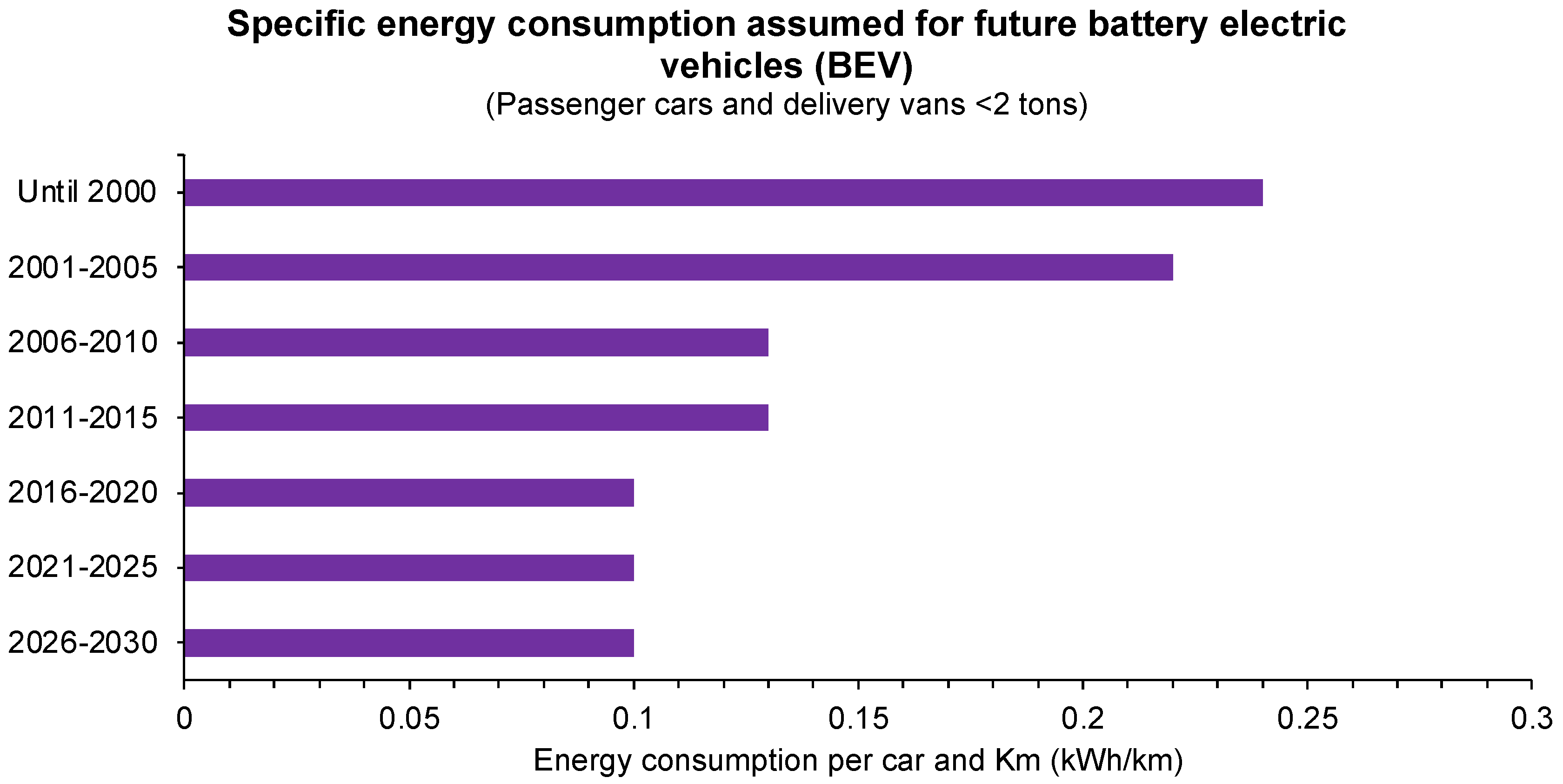
Moreover, Xiong et al. [42] that studied the Chinese case complement the vision of Vilchez and Jochem [41] and Ajanovic and Haas [13]. According to the authors, the BEVs decrease greenhouse effects and energy consumption. This point of view that BEVs can reduce energy consumption is supported by European Environment Agency [74]. According to the agency, the average mass of BEVs increased from 1200 kg in 2010 to 1700 kg in 2019, while average energy consumption decreased from 264 Wh/km to 150 Wh/km, indicating that BEVs have become more efficient. Indeed, the reduction of energy by BEVs was predicted by Nielsen and Jørgensen [75], where according to the authors, the consumption of energy from BEVs will be 0.10 (kWh/km) between 2016 and 2030 (see Figure 13 below).

Indeed, to confirm the capacity of BEVs to reduce energy consumption, we realise a model regression (see Table 10 above), and the results confirmed the visions of Xiong et al. [40] and the European Environment Agency [74], although the result is minimal. Therefore, the BEVs can decrease energy consumption and, consequently, environmental degradation. However, the reduction in the energy consumption caused by BEVs is not enough to mitigate the GHGs in the European region due to the low participation of BEVs in the fleet. For this reason, that final energy consumption is still able to increase GHG emissions.

This field of research is in an exploratory stage of development. Nevertheless, this investigation contributes to the literature with a macroeconomic analysis of the impact of BEVs on GHGs. However, more studies are necessary to deepen the knowledge about the research topic. Therefore, macroeconomic studies should be directed to identify the relationship between BEVs, renewable energy consumption, and GHG emissions. Thus, we can confirm the possible explanation of Vilchez and Jochem [41] and Ajanovic and Haas [13] that the capacity of BEVs to decrease GHG emissions is related to the consumption of energy. In the next section, we will present this study’s conclusions and policy implications.

6. Conclusions and Policy Implications

This analysis explored the effect of BEVs on GHG emissions in a panel of twenty-nine countries from the EU from 2010 to 2020. This study is kick-off regarding the impact of BEVs on GHGs and other aspects such as energy consumption in a macroeconomic and econometric aspect. Indeed, this investigation is in the early stages of maturation and will supply a solid foundation for second-generation research regarding this topic.

The MM-QR was used as the main model, while the OLS with fixed effects was used to verify the robustness of the results. The results from the preliminary tests indicated (i) the variables are not normally distributed, (ii) low multicollinearity between the variables, (iii) presence of cross-section dependence, (iv) variables LnGDP and LnENERGY, without and with the trend, are stationary or I (1), (v) the variables LnGHGs and LnBEVs, without and with the trend, are borderline I (0) and I (1) order of integration, (vi) non-presence of cointegration between the variables LnGDP and LnENERGY, and (vii) presence of fixed effects in the model.

The results from the MM-QR indicates that in all three quantiles, the variable LnGDP causes a positive impact on LnGHGs. In the 50th and 75th quantiles, the variable LnENERGY also causes a positive effect on the dependent variable. Hence, both economic development and energy consumption increase the emissions of GHGs in European Union countries. However, the variable LnBEVs in the 25th, 50th, and 75th quantiles results in a negative impact on the variable LnGHGs, meaning that the battery electric vehicles are capable of mitigating GHGs emissions. Moreover, the results from the OLS with fixed effects indicated that the variable LnGDP has a negative impact on the variable LnGHGs; therefore, it is possible to conclude that economic development mitigates the emissions of GHGs. This finding contradicts the results from the quantile regression. The variable LnENERGY causes a positive impact on the variable LnGHGs, indicating that energy consumption contributes to an increase in GHGs emissions. In contrast, the variable LnBEVs causes negative impacts, which are in line with the results from the quantile regression.

The capacity of economic growth and the final energy consumption to increase the GHGs could be related to the dependence of European countries on energy consumption from non-renewable energy sources to growth. Therefore, economic activity will positively impact energy consumption and negatively affect the environment. This explanation is widely supported and explored by literature and it was proved in this empirical investigation that economic growth increases the final energy consumption in the EU. Now, the capacity of BEVs to mitigate the GHGs could be related to the low energy consumption of electric cars and consequently decrease the energy consumption. Another possible explanation could be the consumption of energy from renewable energy sources by electric vehicles. Thus, the empirical founds of this investigation answered our central question but led us to new questions, such as Do BEVs can increase the consumption of renewable energy, as mentioned by Vilchez and Jochem [41] and Ajanovic and Haas [13])? As the manufacturers say, is the production chain of BEVs (100%) sustainable and clean? These questions need to be answered to understand how the BEVs interact with energy, the economy, and the environment.

In the face of this discovery, another question arises. What are the possible policy implications of this study? This research is motivated not only by the BEVs impacts on emissions but also by the policy implications for the EU to increase the commercialisation of BEV vehicles and decrease the GHGs emissions. Therefore, we recommend the potential policy measures supporting the insertion of BEVs focus on: (i) an intense market penetration; (ii) investments in network and private charging infrastructure; (iii) specific and efficient emission regulations; (iv) technological development (e.g., fast charging; longevity of batteries); (v) additional financial incentives (e.g., feed-in tariffs; fiscal incentives; battery costs); (vi) integration between energy supply and transport sector; (vii) domestic policies considering geographical issues; and (viii) consumer acceptance of BEVs. Moreover, although the EU has supported a more sustainable transport system, accelerating the adoption of BEVs still requires effective political planning in the short, medium, and long term to net-zero pledges emissions. Thus, to achieve the EU targets of decarbonising the energy sector, the BEV has been considered an important technology to reduce GHG emissions. Finally, this research topic can open a channel of policy discussion between industry, government, and researchers, as a crucial step towards ensuring that BEVs provide a climate change mitigation pathway in the region.

7. Limitations of the Study

This investigation is not free of limitations during the process of investigation. The study modelled GHG emissions against major economic determinants, including the BEVs, GDP per capita, and energy consumption. While these variables are a significant contributor to GHG emissions, including renewable energy policies, incentive policies for electric cars, and globalisation index could bring more robustness to the model. However, as we have data until 2018 for the variable globalisation index at KOF Globalisation Index, and until 2019 for the variables renewable energy policies and incentive policies for electric cars at International Energy Agency (IEA)-Policy database, this investigation did not include these variables. Another limitation of this investigation is the lack of macroeconomic data on the ecological footprint of all production chains of electric cars. If this data were available, this investigation could realise a robustness verification to confirm if electric cars decrease the GHG emissions in the EU.

Moreover, another limitation of this study is the impossibility of including dummies in the model. This restriction is due to the short period that this investigation has used. However, these dummies could represent shocks or outliers in the EU countries (e.g., economic, financial, political, social crises, economic growth, etc.). Therefore, these dummies could also bring more robustness to the model. Indeed, these limitations mentioned above are normal in an investigation in the early stages of maturation. Then, as mentioned in the conclusions section, it is necessary to develop second-generation research regarding this topic to overcome these limitations. Despite the limitations mentioned above, the study allows us to draw meaningful conclusions in terms of economic and energy policy. In this context, government policy should encourage electric batteries to reduce greenhouse effects and improve air quality. On the other hand, the European economy must continue implementing green growth practices.

References

1. Meierrieks, D. Weather shocks, climate change and human health. World Dev. 2021, 138, 105228. [Google Scholar] [CrossRef]
2. Bruhwiler, L.; Basu, S.; Butler, J.H.; Chatterjee, A.; Dlugokencky, E.; Kenney, M.A.; Stanitski, D. Observations of greenhouse gases as climate indicators. Clim. Chang. 2021, 165, 12. [Google Scholar] [CrossRef]
3. Inderwildi, O.; King, S.D. Energy, Transport & the Environment: Addressing the Sustainable Mobility Paradigm; Springer: London, UK, 2012. [Google Scholar]
4. De Souza, L.L.P.; Lora, E.E.S.; Palacio, J.C.E.; Rocha, M.H.; Renó, M.L.G.; Venturini, O.J. Comparative environmental life cycle assessment of conventional vehicles with different fuel options, plug-in hybrid and electric vehicles for a sustainable transportation system in Brazil. J. Clean. Prod. 2018, 203, 444–468. [Google Scholar] [CrossRef]
5. IPCC. AR6 Climate Change 2021: The Physical Science Basis. 2021. Available online: https://www.ipcc.ch/report/ar6/wg1/#FullReport (accessed on 2 December 2021).
6. EEA. New Registrations of Electric Vehicles in Europe. 2021. Available online: https://www.eea.europa.eu/data-and-maps/indicators/proportion-of-vehicle-fleet-meeting-5/assessment (accessed on 2 December 2021).
7. Europa. How are Emissions of Greenhouse Gases by the EU Evolving? 2021. Available online: https://ec.europa.eu/eurostat/cache/infographs/energy/bloc-4a.html (accessed on 2 December 2021).
8. Hawkins, T.R.; Singh, B.; Majeau-Bettez, G.; Strømman, A.H. Comparative Environmental Life Cycle Assessment of Conventional and Electric Vehicles. J. Ind. Ecol. 2013, 17, 53–64. [Google Scholar] [CrossRef]
9. Andersson, Ö.; Börjesson, P. The greenhouse gas emissions of an electrified vehicle combined with renewable fuels: Life cycle assessment and policy implications. Appl. Energy 2021, 289, 116621. [Google Scholar] [CrossRef]
10. Xu, L.; Yilmaz, H.Ü.; Wang, Z.; Poganietz, W.R.; Jochem, P. Greenhouse gas emissions of electric vehicles in Europe considering different charging strategies. Transp. Res. Part D Transp. Environ. 2020, 87, 102534. [Google Scholar] [CrossRef]
11. Helmers, E.; Marx, P. Electric cars: Technical characteristics and environmental impacts. Environ. Sci. Eur. 2012, 24, 14. [Google Scholar] [CrossRef] [Green Version]
12. Tagliaferri, C.; Evangelisti, S.; Acconcia, F.; Domenech, T.; Ekins, P.; Barletta, D.; Lettieri, P. Life cycle assessment of future electric and hybrid vehicles: A cradle-to-grave systems engineering approach. Chem. Eng. Res. Des. 2016, 112, 298–309. [Google Scholar] [CrossRef]
13. Ajanovic, A.; Haas, R. On the environmental benignity of electric vehicles. J. Sustain. Dev. Energy Water Environ. Syst. 2019, 7, 416–431. [Google Scholar] [CrossRef]
14. Bekel, K.; Pauliuk, S. Prospective cost and environmental impact assessment of battery and fuel cell electric vehicles in Germany. Int. J. Life Cycle Assess. 2019, 24, 2220–2237. [Google Scholar] [CrossRef]
15. European Alternative Fuels Observatory (EAFO). Vehicles and Fleet. 2021. Available online: https://www.eafo.eu/ (accessed on 2 December 2021).
16. Hooftman, N.; Oliveira, L.; Messagie, M.; Coosemans, T.; Van Mierlo, J. Environmental analysis of petrol, diesel and electric passenger cars in a Belgian urban setting. Energies 2016, 9, 84. [Google Scholar] [CrossRef]
17. Gryparis, E.; Papadopoulos, P.; Leligou, H.C.; Psomopoulos, C.S. Electricity demand and carbon emission in power generation under high penetration of electric vehicles. A European Union perspective. Energy Rep. 2020, 6, 475–486. [Google Scholar] [CrossRef]
18. Burchart-Korol, D.; Jursova, S.; Folęga, P.; Pustejovska, P. Life cycle impact assessment of electric vehicle battery charging in European Union countries. J. Clean. Prod. 2020, 257, 120476. [Google Scholar] [CrossRef]
19. Wu, Z.; Wang, M.; Zheng, J.; Sun, X.; Zhao, M.; Wanga, X. Life cycle greenhouse gas emission reduction potential of battery electric vehicle. J. Clean. Prod. 2018, 190, 462–470. [Google Scholar] [CrossRef]
20. Sheng, M.S.; Sreenivasan, A.V.; Sharp, B.; Duc, B. Well-to-wheel analysis of greenhouse gas emissions and energy consumption for electric vehicles: A comparative study in Oceania. Energy Policy 2021, 158, 112552. [Google Scholar] [CrossRef]
21. Asghar, R.; Rehman, F.; Ullah, Z.; Qamar, A.; Ullah, K.; Iqbala, K.; Aman, A.; Nawaz, A.A. Electric vehicles and key adaptation challenges and prospects in Pakistan: A comprehensive review. J. Clean. Prod. 2021, 278, 123375. [Google Scholar] [CrossRef]
22. Saqib, M.; Benhmad, F. Does ecological footprint matter for the shape of the environmental Kuznets curve? Evidence from European countries. Environ. Sci. Pollut. Res. 2021, 28, 13634–13648. [Google Scholar] [CrossRef] [PubMed]
23. Koengkan, M.; Fuinhas, J.A.; Silva, N. Exploring the capacity of renewable energy consumption to reduce outdoor air pollution death rate in Latin America and the Caribbean region. Environ. Sci. Pollut. Res. 2021, 28, 1656–1674. [Google Scholar] [CrossRef]
24. Leitão, N.C. The Effects of corruption, renewable energy, trade and CO2 emissions. Economies 2021, 9, 62. [Google Scholar] [CrossRef]
25. Ouédraogo, M.; Peng, D.; Chen, X.; Hashmi, S.H.; Sall, M.I. Dynamic Effect of Oil Resources on Environmental Quality: Testing the Environmental Kuznets Curve Hypothesis for Selected African Countries. Sustainability 2021, 13, 3649. [Google Scholar] [CrossRef]
26. Balsalobre-Lorente, D.; Driha, O.M.; Leitão, N.C.; Murshed, M. The carbon dioxide neutralizing energy innovation on international tourism in EU-5 countries under the prism of the EKC hypothesis. J. Environ. Manag. 2021, 298, 113513. [Google Scholar] [CrossRef]
27. Shahbaz, M.; Sharma, R.; Sinha, A.; Jiao, Z. Analysing nonlinear impact of economic growth drivers on CO2 emissions: Designing an SDG framework for India. Energy Policy 2021, 48, 111965. [Google Scholar] [CrossRef]
28. Simionescu, M. Revised environmental Kuznets Curve in CEE countries. Evidence from panel threshold models for economic sectors. Environ. Sci. Pollut. Res. 2021, 28, 60881–60899. [Google Scholar] [CrossRef] [PubMed]
29. Leitão, N.C.; Balsalobre-Lorente, D.; Cantos-Cantos, J.M. The impact of renewable energy and economic complexity on carbon emissions in BRICS countries under the EKC Scheme. Energies 2021, 14, 4908. [Google Scholar] [CrossRef]
30. Nwani, C. Taking Venezuela back to the sustainability path: The role of financial development and economic integration in low-carbon transition. Nat. Resour. Forum 2021, 45, 37–62. [Google Scholar] [CrossRef]
31. Uzuner, G.; Akadiri, S.S.; Lasisi, T.T. The asymmetric relationship between globalisation, CO2 emissions, and economic growth in Turkey: Implications for environmental policy making. Environ. Sci. Pollut. Res. 2020, 27, 32742–32753. [Google Scholar] [CrossRef]
32. Dogan, E.; Inglesi-Lotz, R. The impact of economic structure to the environmental Kuznets curve (EKC) hypothesis: Evidence from European countries. Environ. Sci. Pollut. Res. 2020, 27, 12717–12724. [Google Scholar] [CrossRef] [PubMed]
33. Ike, N.G.; Usman, O.; Sarkodie, S.A. Testing the role of oil production in the environmental Kuznets curve of foil producing countries: New insights from Method of Moments Quantile Regression. Sci. Total. Environ. 2020, 711, 135208. [Google Scholar] [CrossRef] [PubMed]
34. Badulescu, D.; Badulescu, A.; Simut, R.; Bac, D.; Iancu, E.-A.; Iancu, N. Exploring environmental Kuznets curve. An investigation on EU economies. Technol. Econ. Dev. Econ. 2020, 26, 1–20. [Google Scholar] [CrossRef]
35. Panait, M.; Voica, M.C.; Radulescu, I. Approaches regarding environmental Kuznets curve in the European Union from the perspective of sustainable development. Appl. Ecol. Environ. Res. 2019, 17, 6801–6820. [Google Scholar] [CrossRef]
36. Koengkan, M.; Losekann, L.D.; Fuinhas, J.A. The relationship between economic growth, consumption of energy, and environmental degradation: Renewed evidence from Andean community nations. Environ. Syst. Decis. 2019, 39, 95–107. [Google Scholar] [CrossRef]
37. Destek, M.A.; Ulucak, R.; Dogan, E. Analyzing environmental Kuznets curve for the EU countries: The role of ecological footprint. Environ. Sci. Pollut. Res. 2018, 25, 29387–29396. [Google Scholar] [CrossRef]
38. Grossman, G.; Krueger, A. Environmental impacts of a North American free trade agreement. Natl. Bur. Econ. Res. 1991, 3914. [Google Scholar] [CrossRef]
39. Grossman, G.M.; Krueger, A.B. Economic Growth and the Environment. Q. J. Econ. 1995, 110, 353–377. [Google Scholar] [CrossRef] [Green Version]
40. Zhao, J.; Xi, X.; Na, Q.; Wang, S.; Kadry, S.N.; Kumar, P.M. The technological innovation of hybrid and plug-in electric vehicles for environment carbon pollution control. Environ. Impact Assess. Rev. 2021, 86, 106506. [Google Scholar] [CrossRef]
41. Vilchez, J.J.G.; Jochem, P. Powertrain technologies and their impact on greenhouse gas emissions in key car markets. Transp. Res. Part D Transp. Environ. 2020, 80, 102214. [Google Scholar] [CrossRef]
42. Xiong, S.; Ji, J.; Ma, X. Comparative life cycle energy and GHG emission analysis for BEVs and PHEVs: A case study in China. Energies 2019, 12, 834. [Google Scholar] [CrossRef] [Green Version]
43. Ketenci, N. Environmental Kuznets curve in the presence of structural breaks: New evidence for individual European Countries. Environ. Sci. Pollut. Res. 2021, 28, 31520–31538. [Google Scholar] [CrossRef]
44. Sharma, K.; Bhattarai, B.; Ahmed, S. Aid, Growth, Remittances and Carbon Emissions in Nepal. Energy J. 2019, 40, 1–21. [Google Scholar] [CrossRef]
45. Ardakani, M.K.; Seyedaliakbar, S.M. Impact of energy consumption and economic growth on CO2 emission using multivariate regression. Energy Strat. Rev. 2019, 26, 100428. [Google Scholar] [CrossRef]
46. Faustino, H.C.; Leitão, N.C. Fragmentation in the automobile manufacturing industry: Evidence from Portugal. J. Econ. Stud. 2011, 38, 287–300. [Google Scholar] [CrossRef]
47. Leitão, N.C. Testing the role of trade on carbon dioxide emissions in Portugal. Economies 2021, 9, 22. [Google Scholar] [CrossRef]
48. Leitão, N.C.; Balogh, J.M. The impact of intra-industry trade on carbon dioxide emissions: The case of the European Union. Agric. Econ. Czech 2020, 66, 203–214. [Google Scholar] [CrossRef]
49. Ferreira, E.; Fuinhas, J.A.; Moutinho, V. An investigation of the environmental Kuznets relationship in BRICS countries at a sectoral economic level. Energy Syst. 2021. [Google Scholar] [CrossRef]
50. Go, Y.H.; Lau, L.S.; Liew, F.M.; Senadjki, A. A transport environmental Kuznets curve analysis for Malaysia: Exploring the role of corruption. Environ. Sci. Pollut. Res. 2021, 28, 3421–3433. [Google Scholar] [CrossRef] [PubMed]
51. Xu, B.; Sharif, A.; Shahbaz, M.; Dong, K. Have electric vehicles effectively addressed CO2 emissions? Analysis of eight leading countries using quantile-on-quantile regression approach. Sustain. Prod. Consum. 2021, 27, 1205–1214. [Google Scholar] [CrossRef]
52. Braun, A.; Rid, W. Energy consumption of an electric and an internal combustion passenger car. A comparative case study from real-world data on the Erfurt circuit in Germany. Transp. Res. Procedia 2017, 27, 468–475. [Google Scholar] [CrossRef]
53. Ozcan, C.C.; Bekun, F.V.; Nazlioglu, S. Tourism-induced pollutant emissions in Mediterranean countries: Evidence from panel causality analysis. Int. Soc. Sci. J. 2021, 71, 261–281. [Google Scholar] [CrossRef]
54. Eurostat. Energy Statistics-An Overview. 2021. Available online: https://ec.europa.eu/eurostat/statistics-explained/index.php?title=Energy_statistics_-_an_overview#Final_energy_consumption (accessed on 2 December 2021).
55. World Bank Open Database. 2021. Available online: https://www.worldbank.org/en/home (accessed on 3 December 2021).
56. Eurostat. Final Energy Consumption by Sector. 2021. Available online: https://ec.europa.eu/eurostat/databrowser/product/page/TEN00124 (accessed on 2 December 2021).
57. Machado, J.A.; Silva, J.S. Quantiles via moments. J. Econom. 2019, 213, 145–173. [Google Scholar] [CrossRef]
58. Canay, I.A. A simple approach to quantile regression for panel data. Econom. J. 2011, 14, 368–386. [Google Scholar] [CrossRef]
59. Lamarche, C. Robust penalised regression estimation for panel data. J. Econom. 2020, 157, 396–408. [Google Scholar] [CrossRef]
60. Koenker, R. Quantile regression for longitudinal data. J. Multivar. Anal. 2004, 91, 74–89. [Google Scholar] [CrossRef] [Green Version]
61. Usman, O.; Bekun, F.V.; Ike, G.N. Democracy and tourism demand in European countries: Does environmental performance matter? Environ. Sci. Pollut. Res. 2020, 27, 38353–38359. [Google Scholar] [CrossRef]
62. Hao, L.; Niaman, D.Q. Quantile-regression Model and Estimation. In Quantile Regression; Hao, L., Niaman, D.Q., Eds.; SAGE Publications: Thousand Oaks, CA, USA, 2007; pp. 22–42. [Google Scholar]
63. Fuinhas, J.A.; Koengkan, M.; Santiago, R. Physical Capital Development and Energy Transition in Latin America and the Caribbean; Elsevier: Amsterdam, The Netherlands, 2021; pp. 1–224. [Google Scholar] [CrossRef]
64. Shapiro, S.S.; Wilk, M.B. An analysis of variance test for normality (complete samples). Biometrika 1965, 52, 591–611. [Google Scholar] [CrossRef]
65. D’Agostino, R.B.; Belanger, A.; D’Agostino, R.B., Jr. A suggestion for using powerful and informative tests of normality. Am. Stat. 1990, 44, 316–321. [Google Scholar] [CrossRef]
66. Belsley, D.A.; Kuh, E.; Welsch, R.E. Regression Diagnostics: Identifying Influential Data and Sources of Collinearity; Wiley: New York, NY, USA, 1980. [Google Scholar] [CrossRef]
67. Pesaran, M.H. General Diagnostic Tests for Cross-Section Dependence in Panels. In Cambridge Working Papers in Economics; The University of Cambridge: Cambridge, UK, 2004; n. 0435. [Google Scholar] [CrossRef]
68. Pesaran, M.H. A simple panel unit root test in the presence of cross-section dependence. J. Appl. Econom. 2007, 22, 256–312. [Google Scholar] [CrossRef] [Green Version]
69. Westerlund, J. Testing for error correction in panel data. Oxf. Bull. Econ. Stat. 2007, 69, 709–748. [Google Scholar] [CrossRef] [Green Version]
70. Hausman, J.A. Specification tests in econometrics. Econometrica 1978, 46, 1251–1271. [Google Scholar] [CrossRef] [Green Version]
71. Koengkan, M.; Fuinhas, J.A. Is gender inequality an essential driver in explaining environmental degradation? Some empirical answers from the CO2 emissions in European Union countries. Environ. Impact Assess. Rev. 2021, 90, 106619. [Google Scholar] [CrossRef]
72. Mendonça, A.K.S.; Barni, G.A.C.; Moro, L.F.; Bornia, A.C.; Kupek, E.; Fernandes, L. Hierarchical modeling of the 50 largest economies to verify the impact of GDP, population and renewable energy generation in CO2 emissions. Sustain. Prod. Consum. 2020, 20, 8–67. [Google Scholar] [CrossRef]
73. Nawaz, M.A.; Hussain, M.S.; Kamran, H.W.; Ehsanullah, S.; Kupek, E.; Maheen, R.; Shair, F. Trilemma association of energy consumption, carbon emission, and economic growth of BRICS and OECD regions: Quantile regression estimation. Environ. Sci. Pollut. Res. 2020, 28, 16014–16028. [Google Scholar] [CrossRef] [PubMed]
74. European Environment Agency. Primary and Final Energy Consumption in Europe. 2021. Available online: https://www.eea.europa.eu/data-and-maps/indicators/final-energy-consumption-by-sector-13/assessment (accessed on 2 December 2021).
75. Nielsen, H.L.; Jørgensen, K. Electric Vehicles and Renewable Energy in the Transport Sector–Energy System Consequences; Risø National Laboratory: Roskilde, Denmark, 2000; pp. 1–82. [Google Scholar]
Figure 1. Greenhouse gas emissions in EU between 1990 and 2019. The authors created this figure with data from EEA [6].
Sustainability 13 13611 g001
Figure 2. GHG emissions by sector in EU, 2018. The authors created this figure with data from Europa [7].
Sustainability 13 13611 g002
Figure 3. GHG emissions by aggregated sector in EU between 1990 and 2018. The authors created this figure with data from EEA [6].
Sustainability 13 13611 g003
Figure 4. New BEVs registered in the EU-27, Iceland, Norway, and the United Kingdom, between 2010 and 2019. The authors created this figure with data from EEA [6].
Sustainability 13 13611 g004
Figure 5. Newly registered BEVs in 2019 by country. The authors created this figure with data from EEA [6].
Sustainability 13 13611 g005
Figure 6. Total number of BEVs in the fleet of the European Union between 2010 and 2020. The authors created this figure with data from European Alternative Fuels Observatory (EAFO) [15].
Sustainability 13 13611 g006
Figure 7. Total number of BEVs by country in 2020. The authors created this figure with data from European Alternative Fuels Observatory (EAFO) [15].
Sustainability 13 13611 g007
Figure 8. Conceptual framework. The authors created this figure.
Sustainability 13 13611 g008
Figure 9. Quantile estimate: Shaded areas are (95%) confidence bands for the quantile regression estimates. The vertical axis shows the elasticities of the explanatory variables. The horizontal lines depict the conventional (95%) confidence intervals for the OLS coefficient.
Sustainability 13 13611 g009
Figure 10. Summary of the variable’s effect. The authors created this figure.
Sustainability 13 13611 g010
Figure 11. Final energy consumption by fuel in EU between 1990 and 2019. The authors created this figure with data from European Environment Agency [74].
Sustainability 13 13611 g011
Figure 12. Final energy consumption by fuel in EU countries in 2019. The authors created this figure with data from European Environment Agency [74].
Sustainability 13 13611 g012
Figure 13. Specific energy consumption is assumed for future battery electric vehicles (BEVs). The authors created this figure with data from Nielsen and Jørgensen [75].
Sustainability 13 13611 g013